README

Spower Provides a general purpose simulation-based power analysis API for routine and customized simulation experimental designs. The package focuses exclusively on Monte Carlo simulation experiment variants of (expected) prospective power analyses, criterion analyses, compromise analyses, sensitivity analyses, and a priori/post-hoc analyses. The default simulation experiment functions defined within the package provide stochastic variants of the power analysis subroutines in GPower 3.1 (Faul, Erdfelder, Buchner, and Lang, 2009), along with various other parametric and non-parametric power analysis applications (e.g., mediation analyses) and support for Bayesian power analysis by way of Bayes factors or posterior probability evaluations. Additional functions for building empirical power curves, reanalyzing simulation information, and for increasing the precision of the resulting power estimates are also included, each of which utilize similar API structures. For further details see the associated publication in Chalmers (2025).

Installation

install.packages("Spower")

To install the development version of the Spower package, you need to install the remotes package then the Spower package.

install.packages("remotes")
remotes::install_github("philchalmers/Spower")

Quick Start

Spower requires only two components: an available function used to generate exactly one simulation experiment that returns one or more p-values given the null hypothesis of interest (or alternative criteria that return logical indicators or posterior probabilities), and the use of either Spower() or SpowerCurve() to perform the desired prospective/post-hoc, a priori, sensitivity, compromise, or criterion power analysis.

For example, the built-in p_t.test() function performs t-tests using various inputs, where below a sample size of \(N=200\) is supplied (n = 100 per group) and a Cohen’s \(d\) of .5 (a so-called “medium” effect). This returns a single \(p\)-value given the null hypotheses of no mean difference, which in this single case returns a ‘surprising’ result given this null position tested.

library(Spower)
p_t.test(n=100, d=0.5)
## [1] 0.001231514

To evaluate the prospective power of this test simply requires passing the simulation function to Spower(), which will perform this experiment with 10,000 independent replications, collecting and summarizing all relevant information for the power analysis.

set.seed(42)
p_t.test(n=100, d=0.5) |> Spower()

##
## Execution time (H:M:S): 00:00:02
## Design conditions: 
##
## # A tibble: 1 × 4
##       n     d sig.level power
##   <dbl> <dbl>     <dbl> <lgl>
## 1   100   0.5      0.05 NA   
## 
## Estimate of power: 0.943
## 95% Confidence Interval: [0.938, 0.947]

Alternatively, for a priori and sensitive analyses, the respective input to the simulation function must be set to NA, while within Spower() the target power rate must be included along with a suitable search interval range. Below the target power is set to \(1-\beta = .95\), while the associated \(n\) is suspected to lay somewhere within the boundary \([50,300]\).

set.seed(01123581321)

# estimate the require n value to achieve a power of 1 - beta = .95 
p_t.test(n=NA, d=0.5) |> Spower(power=.95, interval=c(50, 300))

## Iter: 56; Median = 101; E(f(x)) = 0.00; Total.reps = 11000; k.tol = 2; Pred = 103.4
##
## Execution time (H:M:S): 00:00:05
## Design conditions: 
## 
## # A tibble: 1 × 4
##       n     d sig.level power
##   <dbl> <dbl>     <dbl> <dbl>
## 1    NA   0.5      0.05  0.95
## 
## Estimate of n: 103.4
## 95% Predicted Confidence Interval: [101.5, 105.4]

Estimated power curves

To generate suitable power-curves for any given simulation or power analysis criteria, the simulation experiment can be passed to SpowerCurve() (or to SpowerBatch() first, and then to SpowerCurve()). This function contains a similar specification structure to Spower(), however differs in that the arguments to vary are explicitly passed as named vectors to SpowerCurve(). Below is an example varying sample size (n), while the next example varies both n and the effect size d.

set.seed(8675309) # Jenny Jenny
p_t.test(d=0.2) |> SpowerCurve(n=seq(50, 550, by=100))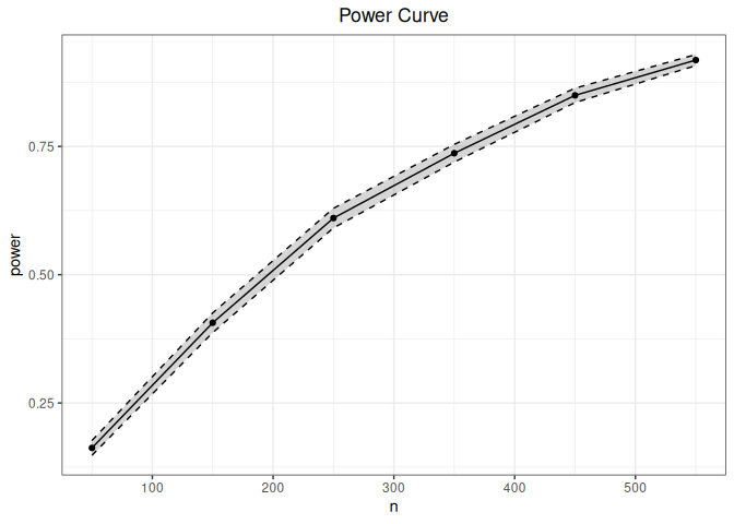

p_t.test() |> SpowerCurve(n=seq(50, 350, by=50), d=c(.2, .3, .4, .5))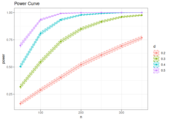

Vignettes

The package currently contains a vignette demonstrating several of the examples from the GPower 3.1 manual, providing simulation-based replications of the same analyses, as well other vignettes showing more advanced applications of the package (ROPEs, Bayesian power analyses, precision criterion, Type S/M errors, etc).

Getting Help or Reporting an Issue

How to Contribute

If you have a simulation experiment you’d like to contribute in the form of either

# returns a p-value, P(D|H0)
p_yourSimulation()

# returns a posterior probability, P(H1|D)
pp_yourSimulation()

# returns a logical (more complex experiments, perhaps involing ROPEs)
l_yourSimulation()