
The radsafer package was developed to provide:
general functions helpful in the practice of radiation safety, for example, decay-corrections
easy access to radionuclide data from the RadData
package
functions for instrumentation and radiation transport modeling
Related functions are identified as members of these families:
decay corrections
radionuclides
radiation measurements
mcnp tools
and a few stand alone functions
Radsafer includes several functions to manage radioactive decay corrections:
dk_correct provides decay-correction of single radionuclides. (Radioactive in-growth is not accounted for.)
dk_correct(RN_select = "Sr-90",
           date1 = "2015-01-01", #Original activity date
           date2 = c("2025-01-01","2035-01-01"), #Decay to these dates
           A1 = 10000) #Original activity (arbitrary units)
#>     RN half_life units decay_mode
#>  Sr-90     28.79     y         B-
#>
#>     RN RefValue    RefDate   TargDate dk_value
#>  Sr-90    10000 2015-01-01 2025-01-01 7860.079
#> Sr-90 10000 2015-01-01 2035-01-01 6178.491dk_correct(half_life = 10, #10 something - need unit
time_unit = "y",#unit is years
date1 = "2010-01-01") #original date is identified
#> half_life RefValue RefDate TargDate dk_value
#> 10 1 2010-01-01 2026-07-14 0.3179556
# Since date2 is not identified, it defaults to the computer's system date "today".dk_correct(RN_select = "Cs-137",
date1 = "2026-01-01", #known activity on this date
date2 = c("2016-01-01","2006-01-01"), #find activity on these earlier dates
A1 = 3000) #original activity (arbitrary units)
#> RN half_life units decay_mode
#> Cs-137 30.1671 y B-
#>
#> RN RefValue RefDate TargDate dk_value
#> Cs-137 3000 2026-01-01 2016-01-01 3775.032
#> Cs-137 3000 2026-01-01 2006-01-01 4749.991dk_time(half_life = 5730, A0 = 14, A1 = 1)
#> [1] 21816.14
RN_find_parent("Po-210")
#> RN
#> 1 At-210
#> 2 Bi-210RadDataPlot an emission spectrum
RN_plot_spectrum(
  desired_RN = c("Pu-238", "Pu-239", "Am-241"), rad_type = "A",
  photon = FALSE, prob_cut = 0.01, log_plot = 0)
RN_plot_spectrum(
     desired_RN = c("Sr-90", "Y-90"), rad_type = "B-")
RN_plot_spectrum(desired_RN = c("Co-60", "Ba-137m"), rad_type = "G")
Search by alpha, beta, photon or use the general screen option.
# tight energy limits around 1 MeV
search_results <- RN_search_phot_by_E(E_min = 0.99,
                    E_max = 1.01,
# half-life between 13 and 15 minutes (convert from seconds)
                    min_half_life_seconds = 13 * 60,
                    max_half_life_seconds = 15 * 60,
# only branches with probabilities >= 10%
                    min_prob = 0.1)

RN_plot_spectrum(desired_RN = search_results$RN, rad_type = "G", prob_cut = 0.1)
#> [1] "No matches"disk_to_disk_solid_angle(r.source = 45/2, gap = 20, r.detector = 12.5, runs = 1e4, plot.opt = "2d")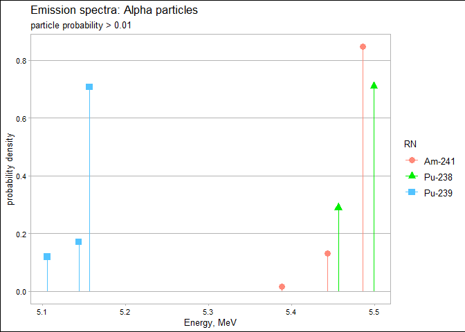
#>    mean_eff         SEM
#>  0.05132699 0.002208406

scaler_sim(true_bkg = 50, true_samp = 10, ct_time = 20, trials = 1e5)
rate_meter_sim(cpm_equilibrium = 270, meter_scale_increments = seq(100, 1000, 20))
mcnp_sdef_erg_line("Co-60", photon = TRUE, cut = 0.01, erg.dist = 13)
#> # A tibble: 6 × 6
#>   RN    code_AN E_MeV     prob code_num is_photon
#>   <chr> <chr>   <dbl>    <dbl>    <dbl> <lgl>
#> 1 Co-60 G       0.347 0.000075        1 TRUE
#> 2 Co-60 G       0.826 0.000076        1 TRUE
#> 3 Co-60 G       1.17  0.998           1 TRUE
#> 4 Co-60 G       1.33  1.000           1 TRUE
#> 5 Co-60 G       2.16  0.000012        1 TRUE
#> # ℹ 1 more row

mcnp_matrix_rotations("z", 30)
#> [1]  0.8660254  0.5000000  0.0000000 -0.5000000  0.8660254  0.0000000
#> [7] 0.0000000 0.0000000 1.0000000If you encounter a clear bug, please file an issue with a minimal reproducible example on GitHub.