The BerkeleyForestsAnalytics package (BFA) is a suite of
open-source R functions designed to produce standard metrics from forest
inventory data. The package is designed and maintained by Berkeley
Forests – a research unit in University of California Berkeley’s Rausser
College of Natural Resources. Berkeley Forests manages a network of six
forest properties to develop and test management strategies that promote
the resilience of working forest lands. This package is built to analyze
the data generated by Berkeley Forests’ continuous forest inventories.
The basic design is a gridded network of nested, fixed radius plots
where trees are measured and tagged.
BFA’s overarching goal is to minimize potential inconsistencies introduced by the algorithms used to compute and summarize core forest metrics. It was explicitly designed to address common analytical issues including: 1) Unit conversion errors; 2) Missing zeros; 3) Undocumented NA handling; 4) Imprecise scaling; and 5) Ad hoc application of allometric equations. In short, our objective is to obtain consistent results from the same data. We developed BFA using Base R code to help reduce the frequency of minor code maintenance. All applications can accommodate data recorded using imperial units (typical for forest management) or metric units (typical for forest science). We also provide a plethora of custom warnings when our error checking routines encounter unexpected inputs or formats.
- Installation instructions
- Vignette
- Citation instructions
- Copyright notice
- Tree biomass and carbon estimates (NSVB framework)
- Stand density index
- Forest composition and structure compilations
- Surface and ground fuel load estimations
- Further data summarization
- Background information for tree biomass and carbon estimations (NSVB framework)
- Background information for stand density index
- Background information for surface and ground fuel load calculations
- Background information for further data summarization
- Contact information
The GitHub version may be slightly ahead of the CRAN version of
BerkeleyForestsAnalytics. If CRAN and GitHub have different
version numbers, the GitHub version represents a public-ready,
late-stage development version of the package that is safe to install,
whereas the CRAN version is the formally submitted and approved
release.
To install the BerkeleyForestsAnalytics package from
CRAN (current version 4.0.0):
install.packages("BerkeleyForestsAnalytics")
library(BerkeleyForestsAnalytics)
To install the BerkeleyForestsAnalytics package from
GitHub (current version 4.0.0):
# install and load devtools
install.packages("devtools")
library(devtools)
# install and load BerkeleyForestsAnalytics
devtools::install_github('kearutherford/BerkeleyForestsAnalytics')
library(BerkeleyForestsAnalytics)# install and load BerkeleyForestsAnalytics
# and request vignettes
devtools::install_github('kearutherford/BerkeleyForestsAnalytics', build_vignettes = TRUE)
library(BerkeleyForestsAnalytics)To access the Vignette for BerkeleyForestsAnalytics:
# Option 1:
browseVignettes("BerkeleyForestsAnalytics")

# Option 2:
vignette("BerkeleyForestsAnalytics", package = "BerkeleyForestsAnalytics")Cite the version used in your project (which may differ from the version in the citation below).
citation("BerkeleyForestsAnalytics")## To cite package 'BerkeleyForestsAnalytics' in publications use:
##
## Kea Rutherford, Danny Foster, John Battles (2026).
## _BerkeleyForestsAnalytics, version 4.0.0_. Battles Lab: Forest
## Ecology and Ecosystem Dynamics, University of California, Berkeley.
## <https://github.com/kearutherford/BerkeleyForestsAnalytics>.
##
## A BibTeX entry for LaTeX users is
##
## @Manual{,
## title = {BerkeleyForestsAnalytics, version 4.0.0},
## author = {{Kea Rutherford} and {Danny Foster} and {John Battles}},
## organization = {Battles Lab: Forest Ecology and Ecosystem Dynamics, University of California, Berkeley},
## year = {2026},
## url = {https://github.com/kearutherford/BerkeleyForestsAnalytics},
## }Copyright ©2024. The Regents of the University of California (Regents). All Rights Reserved. Permission to use, copy, modify, and distribute this software and its documentation for educational, research, and not-for-profit purposes, without fee and without a signed licensing agreement, is hereby granted, provided that the above copyright notice, this paragraph and the following two paragraphs appear in all copies, modifications, and distributions.
IN NO EVENT SHALL REGENTS BE LIABLE TO ANY PARTY FOR DIRECT, INDIRECT, SPECIAL, INCIDENTAL, OR CONSEQUENTIAL DAMAGES, INCLUDING LOST PROFITS, ARISING OUT OF THE USE OF THIS SOFTWARE AND ITS DOCUMENTATION, EVEN IF REGENTS HAS BEEN ADVISED OF THE POSSIBILITY OF SUCH DAMAGE.
REGENTS SPECIFICALLY DISCLAIMS ANY WARRANTIES, INCLUDING, BUT NOT LIMITED TO, THE IMPLIED WARRANTIES OF MERCHANTABILITY AND FITNESS FOR A PARTICULAR PURPOSE. THE SOFTWARE AND ACCOMPANYING DOCUMENTATION, IF ANY, PROVIDED HEREUNDER IS PROVIDED “AS IS”. REGENTS HAS NO OBLIGATION TO PROVIDE MAINTENANCE, SUPPORT, UPDATES, ENHANCEMENTS, OR MODIFICATIONS.
The BiomassNSVB function follows the new national-scale
volume and biomass (NSVB) framework to estimate above-ground wood, bark,
branch, merchantable, stump, and foliage tree biomass and carbon. This
function allows for biomass and carbon estimates of all Forest Inventory
and Analysis (FIA) species. See Background
information for tree biomass estimations (NSVB framework) below for
further details.
BiomassNSVB( ) data A dataframe or tibble. Each row must be an
observation of an individual tree. Must have at least these columns
(column names are exact):
division: Must be a character variable. Describes the Ecological Division in which the data were collected (see Ecological Divisions and Provinces section in “Background information for tree biomass estimates (NSVB framework)” below).
province: Must be a character variable. Describes the Ecological Province (within the Ecological Division) in which the data were collected (see Ecological Divisions and Provinces section in “Background information for tree biomass estimates (NSVB framework)” below).
site: Must be a character variable. Describes the broader location or forest where the data were collected.
plot: Must be a character variable. Identifies the plot in which the individual tree was measured.
stand_org: Must be a character variable. Specifies whether the stand origin is planted (1) or natural (0). Only necessary to include this column if the input data has slash pine (SPCD=111) and/or loblolly pine (SPCD=131). If the column is required, it is only necessary to correctly define the stand origin for the particular plots that include those two speices (you can put 1, 0, or simply NA for the plots without those two species).
exp_factor: Must be a numeric variable. The expansion factor specifies the number of trees per hectare (or per acre) that a given plot tree represents.
status: Must be a character variable. Specifies whether the individual tree is alive (1) or dead (0).
decay_class: Must be a character variable. For standing dead trees, the decay class should be 1, 2, 3, 4, or 5 (see Decay class code table section in “Background information for tree biomass and carbon estimations” below). For live trees, the decay class should be NA or 0.
species: Must be a character variable. Specifies the species of the individual tree. Must follow FIA naming conventions (download FIADB REF_SPECIES file from HERE for reference).
dbh: Must be a numeric variable. Provides the diameter at breast height (DBH) of the individual tree in either centimeters or inches.
ht1: Must be a numeric variable. Required for trees with or without tops. For trees with tops (top = Y), ht1 is the measured height of the individual tree in either meters or feet. For trees without tops (top = N), ht1 is the estimated height of the tree with its top in either meters or feet (in this case, ht1 would likely be estimated using regional allometric equations).
ht2: Must be a numeric variable. Only required for trees without tops (top = N). For trees without tops, ht2 is the “actual height” (i.e., measured height) of the individual tree in either meters or feet.
crown_ratio: Must be a numeric variable. Provides the live crown ratio of the individual tree (between 0 and 1).
top: Must be a character variable. Specifies whether the individual tree has its top, yes (Y) or no (N).
cull: Must be a numeric variable. Provides the percent wood cull of the individual tree (between 0 and 100).
input_units Not a variable (column) in the provided
dataframe or tibble. Specifies (1) whether the input dbh, ht1, and ht2
variables were measured using metric (centimeters and meters) or
imperial (inches and feet) units; and (2) whether the input expansion
factor is in metric (stems per hectare) or imperial (stems per acre)
units. Must be set to either “metric” or “imperial”. The default is set
to “metric”.
output_units Not a variable (column) in the provided
dataframe or tibble. Specifies whether results will be given in metric
(kilograms or megagrams per hectare) or imperial (US tons or US tons per
acre) units. Must be set to either “metric” or “imperial”. The default
is set to “metric”.
results Not a variable (column) in the provided
dataframe or tibble. Specifies whether the results will be summarized by
tree, by plot, by plot as well as species, by plot as well as status
(live/dead), or by plot as well as species and status. Must be set to
either “by_tree”, “by_plot”, “by_species”, “by_status”, or “by_sp_st”.
The default is set to “by_plot”.
Depends on the results setting:
by_tree: a list with two components: (1) total run time for the function and (2) a dataframe with tree-level biomass and carbon estimates.
by_plot: a list with two components: (1) total run time for the function and (2) a dataframe with plot-level biomass and carbon estimates.
by_species: a list with two components: (1) total run time for the function and (2) a dataframe with plot-level biomass and carbon estimates, further summarized by species.
by_status: a list with two components: (1) total run time for the function and (2) a dataframe with plot-level biomass and carbon estimates, further summarized by status.
by_sp_st: a list with two components: (1) total run time for the function and (2) a dataframe with plot-level biomass and carbon estimates, further summarized by species as well as by status.
How to interpret column names of the output dataframe:
# investigate input dataframe
nsvb_demo
## division province site plot exp_factor status decay_class species dbh ht1
## 1 M260 M261 SEKI 1 50 1 <NA> 202 10.3 5.1
## 2 M260 M261 SEKI 1 50 0 2 15 44.7 26.4
## 3 M260 M261 SEKI 1 50 1 <NA> 202 19.1 8.0
## 4 M260 M261 SEKI 1 50 1 <NA> 202 32.8 23.3
## 5 M260 M261 SEKI 1 50 0 3 15 13.8 11.1
## 6 M260 M261 SEKI 2 50 1 <NA> 15 20.2 8.5
## 7 M260 M261 SEKI 2 50 1 <NA> 15 31.7 22.3
## 8 M260 M261 SEKI 2 50 1 <NA> 15 13.1 9.7
## 9 M260 M261 SEKI 2 50 0 3 15 26.3 15.6
## 10 M260 M261 YOMI 1 50 1 <NA> 202 10.7 5.5
## 11 M260 M261 YOMI 1 50 1 <NA> 202 40.6 28.4
## 12 M260 M261 YOMI 1 50 1 <NA> 15 20.1 7.9
## 13 M260 M261 YOMI 1 50 1 <NA> 202 33.8 22.3
## 14 M260 M261 YOMI 1 50 1 <NA> 15 12.4 10.8
## 15 M260 M261 YOMI 1 50 1 <NA> 202 22.2 9.5
## 16 M260 M261 YOMI 2 0 <NA> <NA> <NA> NA NA
## ht2 crown_ratio top cull
## 1 NA 0.3 Y 0
## 2 NA NA Y 0
## 3 6.0 0.4 N 10
## 4 NA 0.4 Y 0
## 5 8.2 NA N 0
## 6 NA 0.5 Y 0
## 7 NA 0.4 Y 5
## 8 NA 0.2 Y 0
## 9 NA NA Y 10
## 10 NA 0.6 Y 5
## 11 18.6 0.4 N 0
## 12 NA 0.3 Y 10
## 13 NA 0.3 Y 0
## 14 NA 0.5 Y 0
## 15 NA 0.2 Y 0
## 16 NA NA <NA> NANotice that site = YOMI, plot = 2 is a plot without trees. For all plot-level summaries below, this plot without trees will have 0 biomass/carbon estimates.
Results by tree:
# call the BiomassNSVB() function in the BerkeleyForestsAnalytics package
# keep default input_units (= "metric") and output_units (= "metric")
nsvb_demo1 <- BiomassNSVB(data = nsvb_demo,
                          results = "by_tree")

nsvb_demo1$run_time
## Time difference of 0.12 secshead(nsvb_demo1$dataframe, 3)## division province site plot exp_factor status decay_class species dbh_cm
## 1 M260 M261 SEKI 1 50 0 2 15 44.7
## 2 M260 M261 SEKI 2 50 0 3 15 26.3
## 3 M260 M261 SEKI 1 50 0 3 15 13.8
## ht1_m ht2_m crown_ratio top cull total_wood_kg total_bark_kg total_branch_kg
## 1 26.4 NA NA Y 0 642.71380 202.68561 78.3319204
## 2 15.6 NA NA Y 10 121.63963 15.47473 2.3823889
## 3 11.1 8.2 NA N 0 24.00841 2.94245 0.2660589
## total_ag_kg merch_wood_kg merch_bark_kg merch_total_kg merch_top_kg
## 1 923.73133 619.85693 195.47748 815.33441 82.640438
## 2 139.49675 112.09243 14.26015 126.35259 6.282084
## 3 27.21692 18.11868 2.22061 20.33929 4.928325
## stump_wood_kg stump_bark_kg stump_total_kg foliage_kg total_wood_c
## 1 19.581327 6.1751484 25.756475 0 323.92776
## 2 6.087625 0.7744543 6.862079 0 61.54965
## 3 1.736484 0.2128220 1.949306 0 12.14826
## total_bark_c total_branch_c total_ag_c merch_wood_c merch_bark_c
## 1 102.153545 39.4792879 465.56059 312.407892 98.520652
## 2 7.830212 1.2054888 70.58536 56.718771 7.215638
## 3 1.488880 0.1346258 13.77176 9.168053 1.123629
## merch_total_c merch_top_c stump_wood_c stump_bark_c stump_total_c foliage_c
## 1 410.92854 41.650781 9.868989 3.1122748 12.9812636 0
## 2 63.93441 3.178735 3.080338 0.3918739 3.4722121 0
## 3 10.29168 2.493733 0.878661 0.1076879 0.9863489 0
## calc_bio
## 1 Y
## 2 Y
## 3 YResults summarized by plot:
# call the BiomassNSVB() function in the BerkeleyForestsAnalytics package
# keep default input_units (= "metric"), output_units (= "metric"), and results (= "by_plot")
nsvb_demo2 <- BiomassNSVB(data = nsvb_demo)

nsvb_demo2
## $run_time
## Time difference of 0.07 secs
##
## $dataframe
## site plot total_wood_Mg_ha total_bark_Mg_ha total_branch_Mg_ha total_ag_Mg_ha
## 1 SEKI 1 51.95205 13.31781 6.37886 71.64872
## 2 SEKI 2 23.03188 6.76482 4.32321 34.11992
## 3 YOMI 1 52.54560 8.27765 5.01073 65.83398
## 4 YOMI 2 0.00000 0.00000 0.00000 0.00000
## merch_total_Mg_ha merch_top_Mg_ha stump_total_Mg_ha foliage_Mg_ha
## 1 62.10950 7.04151 2.17434 1.34616
## 2 27.50977 5.28423 1.32592 2.31164
## 3 56.59898 5.11162 2.09854 3.15141
## 4 0.00000 0.00000 0.00000 0.00000
## total_wood_c total_bark_c total_branch_c total_ag_c merch_total_c merch_top_c
## 1 26.40210 6.74768 3.24337 36.39315 31.54092 3.58030
## 2 11.71685 3.44517 2.20310 17.36511 13.99835 2.69221
## 3 27.07615 4.26527 2.58098 33.92240 29.17330 2.63378
## 4 0.00000 0.00000 0.00000 0.00000 0.00000 0.00000
## stump_total_c foliage_c
## 1 1.10521 0.67308
## 2 0.67455 1.15582
## 3 1.08099 1.57570
## 4 0.00000 0.00000Results summarized by plot as well as by species:
# call the BiomassNSVB() function in the BerkeleyForestsAnalytics package
# keep default input_units (= "metric") and output_units (= "metric")
nsvb_demo3 <- BiomassNSVB(data = nsvb_demo,
                          results = "by_species")

nsvb_demo3
## $run_time
## Time difference of 0.07 secs
##
## $dataframe
## site plot species total_wood_Mg_ha total_bark_Mg_ha total_branch_Mg_ha
## 1 SEKI 1 15 33.33611 10.28140 3.92990
## 2 SEKI 1 202 18.61593 3.03641 2.44896
## 3 SEKI 2 15 23.03188 6.76482 4.32321
## 4 SEKI 2 202 0.00000 0.00000 0.00000
## 5 YOMI 1 15 2.73763 0.44978 0.42931
## 6 YOMI 1 202 49.80797 7.82787 4.58142
## 7 YOMI 2 15 0.00000 0.00000 0.00000
## 8 YOMI 2 202 0.00000 0.00000 0.00000
## total_ag_Mg_ha merch_total_Mg_ha merch_top_Mg_ha stump_total_Mg_ha
## 1 47.54741 41.78369 4.37844 1.38529
## 2 24.10131 20.32581 2.66308 0.78905
## 3 34.11992 27.50977 5.28423 1.32592
## 4 0.00000 0.00000 0.00000 0.00000
## 5 3.61671 1.50943 0.29714 0.17173
## 6 62.21726 55.08955 4.81449 1.92681
## 7 0.00000 0.00000 0.00000 0.00000
## 8 0.00000 0.00000 0.00000 0.00000
## foliage_Mg_ha total_wood_c total_bark_c total_branch_c total_ag_c
## 1 0.00000 16.80380 5.18212 1.98070 23.96662
## 2 1.34616 9.59830 1.56556 1.26268 12.42653
## 3 2.31164 11.71685 3.44517 2.20310 17.36511
## 4 0.00000 0.00000 0.00000 0.00000 0.00000
## 5 0.72647 1.39537 0.22925 0.21882 1.84344
## 6 2.42493 25.68078 4.03602 2.36216 32.07896
## 7 0.00000 0.00000 0.00000 0.00000 0.00000
## 8 0.00000 0.00000 0.00000 0.00000 0.00000
## merch_total_c merch_top_c stump_total_c foliage_c
## 1 21.06101 2.20723 0.69838 0.00000
## 2 10.47990 1.37307 0.40683 0.67308
## 3 13.99835 2.69221 0.67455 1.15582
## 4 0.00000 0.00000 0.00000 0.00000
## 5 0.76936 0.15145 0.08753 0.36324
## 6 28.40394 2.48233 0.99346 1.21247
## 7 0.00000 0.00000 0.00000 0.00000
## 8 0.00000 0.00000 0.00000 0.00000Results summarized by plot as well as by status:
# call the BiomassNSVB() function in the BerkeleyForestsAnalytics package
# keep default input_units (= "metric") and output_units (= "metric")
nsvb_demo4 <- BiomassNSVB(data = nsvb_demo,
                          results = "by_status")

nsvb_demo4
## $run_time
## Time difference of 0.07 secs
##
## $dataframe
## site plot total_wood_L_Mg_ha total_wood_D_Mg_ha total_bark_L_Mg_ha
## 1 SEKI 1 18.61593 33.33611 3.03641
## 2 SEKI 2 16.94990 6.08198 5.99108
## 3 YOMI 1 52.54560 0.00000 8.27765
## 4 YOMI 2 0.00000 0.00000 0.00000
## total_bark_D_Mg_ha total_branch_L_Mg_ha total_branch_D_Mg_ha total_ag_L_Mg_ha
## 1 10.28140 2.44896 3.92990 24.10131
## 2 0.77374 4.20409 0.11912 27.14508
## 3 0.00000 5.01073 0.00000 65.83398
## 4 0.00000 0.00000 0.00000 0.00000
## total_ag_D_Mg_ha merch_total_L_Mg_ha merch_total_D_Mg_ha merch_top_L_Mg_ha
## 1 47.54741 20.32581 41.78369 2.66308
## 2 6.97484 21.19214 6.31763 4.97012
## 3 0.00000 56.59898 0.00000 5.11162
## 4 0.00000 0.00000 0.00000 0.00000
## merch_top_D_Mg_ha stump_total_L_Mg_ha stump_total_D_Mg_ha foliage_L_Mg_ha
## 1 4.37844 0.78905 1.38529 1.34616
## 2 0.31410 0.98282 0.34310 2.31164
## 3 0.00000 2.09854 0.00000 3.15141
## 4 0.00000 0.00000 0.00000 0.00000
## total_wood_L_c total_wood_D_c total_bark_L_c total_bark_D_c total_branch_L_c
## 1 9.59830 16.80380 1.56556 5.18212 1.26268
## 2 8.63937 3.07748 3.05366 0.39151 2.14283
## 3 27.07615 0.00000 4.26527 0.00000 2.58098
## 4 0.00000 0.00000 0.00000 0.00000 0.00000
## total_branch_D_c total_ag_L_c total_ag_D_c merch_total_L_c merch_total_D_c
## 1 1.98070 12.42653 23.96662 10.47990 21.06101
## 2 0.06027 13.83585 3.52927 10.80163 3.19672
## 3 0.00000 33.92240 0.00000 29.17330 0.00000
## 4 0.00000 0.00000 0.00000 0.00000 0.00000
## merch_top_L_c merch_top_D_c stump_total_L_c stump_total_D_c foliage_L_c
## 1 1.37307 2.20723 0.40683 0.69838 0.67308
## 2 2.53327 0.15894 0.50094 0.17361 1.15582
## 3 2.63378 0.00000 1.08099 0.00000 1.57570
## 4 0.00000 0.00000 0.00000 0.00000 0.00000Results summarized by plot as well as by species and status:
# call the BiomassNSVB() function in the BerkeleyForestsAnalytics package
# keep default input_units (= "metric") and output_units (= "metric")
nsvb_demo5 <- BiomassNSVB(data = nsvb_demo,
                          results = "by_sp_st")

nsvb_demo5
## $run_time
## Time difference of 0.08 secs
##
## $dataframe
## site plot species total_wood_L_Mg_ha total_wood_D_Mg_ha total_bark_L_Mg_ha
## 1 SEKI 1 15 0.00000 33.33611 0.00000
## 2 SEKI 1 202 18.61593 0.00000 3.03641
## 3 SEKI 2 15 16.94990 6.08198 5.99108
## 4 SEKI 2 202 0.00000 0.00000 0.00000
## 5 YOMI 1 15 2.73763 0.00000 0.44978
## 6 YOMI 1 202 49.80797 0.00000 7.82787
## 7 YOMI 2 15 0.00000 0.00000 0.00000
## 8 YOMI 2 202 0.00000 0.00000 0.00000
## total_bark_D_Mg_ha total_branch_L_Mg_ha total_branch_D_Mg_ha total_ag_L_Mg_ha
## 1 10.28140 0.00000 3.92990 0.00000
## 2 0.00000 2.44896 0.00000 24.10131
## 3 0.77374 4.20409 0.11912 27.14508
## 4 0.00000 0.00000 0.00000 0.00000
## 5 0.00000 0.42931 0.00000 3.61671
## 6 0.00000 4.58142 0.00000 62.21726
## 7 0.00000 0.00000 0.00000 0.00000
## 8 0.00000 0.00000 0.00000 0.00000
## total_ag_D_Mg_ha merch_total_L_Mg_ha merch_total_D_Mg_ha merch_top_L_Mg_ha
## 1 47.54741 0.00000 41.78369 0.00000
## 2 0.00000 20.32581 0.00000 2.66308
## 3 6.97484 21.19214 6.31763 4.97012
## 4 0.00000 0.00000 0.00000 0.00000
## 5 0.00000 1.50943 0.00000 0.29714
## 6 0.00000 55.08955 0.00000 4.81449
## 7 0.00000 0.00000 0.00000 0.00000
## 8 0.00000 0.00000 0.00000 0.00000
## merch_top_D_Mg_ha stump_total_L_Mg_ha stump_total_D_Mg_ha foliage_L_Mg_ha
## 1 4.37844 0.00000 1.38529 0.00000
## 2 0.00000 0.78905 0.00000 1.34616
## 3 0.31410 0.98282 0.34310 2.31164
## 4 0.00000 0.00000 0.00000 0.00000
## 5 0.00000 0.17173 0.00000 0.72647
## 6 0.00000 1.92681 0.00000 2.42493
## 7 0.00000 0.00000 0.00000 0.00000
## 8 0.00000 0.00000 0.00000 0.00000
## total_wood_L_c total_wood_D_c total_bark_L_c total_bark_D_c total_branch_L_c
## 1 0.00000 16.80380 0.00000 5.18212 0.00000
## 2 9.59830 0.00000 1.56556 0.00000 1.26268
## 3 8.63937 3.07748 3.05366 0.39151 2.14283
## 4 0.00000 0.00000 0.00000 0.00000 0.00000
## 5 1.39537 0.00000 0.22925 0.00000 0.21882
## 6 25.68078 0.00000 4.03602 0.00000 2.36216
## 7 0.00000 0.00000 0.00000 0.00000 0.00000
## 8 0.00000 0.00000 0.00000 0.00000 0.00000
## total_branch_D_c total_ag_L_c total_ag_D_c merch_total_L_c merch_total_D_c
## 1 1.98070 0.00000 23.96662 0.00000 21.06101
## 2 0.00000 12.42653 0.00000 10.47990 0.00000
## 3 0.06027 13.83585 3.52927 10.80163 3.19672
## 4 0.00000 0.00000 0.00000 0.00000 0.00000
## 5 0.00000 1.84344 0.00000 0.76936 0.00000
## 6 0.00000 32.07896 0.00000 28.40394 0.00000
## 7 0.00000 0.00000 0.00000 0.00000 0.00000
## 8 0.00000 0.00000 0.00000 0.00000 0.00000
## merch_top_L_c merch_top_D_c stump_total_L_c stump_total_D_c foliage_L_c
## 1 0.00000 2.20723 0.00000 0.69838 0.00000
## 2 1.37307 0.00000 0.40683 0.00000 0.67308
## 3 2.53327 0.15894 0.50094 0.17361 1.15582
## 4 0.00000 0.00000 0.00000 0.00000 0.00000
## 5 0.15145 0.00000 0.08753 0.00000 0.36324
## 6 2.48233 0.00000 0.99346 0.00000 1.21247
## 7 0.00000 0.00000 0.00000 0.00000 0.00000
## 8 0.00000 0.00000 0.00000 0.00000 0.00000The StandDensity function estimates current stand
density index (SDI), maximum SDI, and relative density. See Background information for stand density
index below for further details.
StandDensity( ) tree_data A dataframe or tibble. Each row must be an
observation of an individual tree. Must have at least these columns
(column names are exact):
site: Must be a character variable. Describes the broader location or forest where the data were collected.
plot: Must be a character variable. Identifies the plot in which the individual tree was measured.
exp_factor: Must be a numeric variable. The expansion factor specifies the number of trees per hectare (or per acre) that a given plot tree represents.
status: Must be a character variable. Specifies whether the individual tree is alive (1) or dead (0).
dbh: Must be a numeric variable. Provides the diameter at breast height (DBH) of the individual tree in either centimeters or inches.
subsec_data A dataframe or tibble. Each row must
correspond to an individual site or site/plot. Must have at least these
columns (column names are exact):
site: Must be a character variable. Describes the broader location or forest where the data were collected.
plot: Must be a character variable. This column is OPTIONAL. If all plots within a site are located in the same subsection, this column is not needed. If plots within a site span multiple subsections, this column may be included.
subsection: Must be a numeric variable. Describes the Ecological Subsection in which the data were collected (see Ecological Subsections section in “Background information for stand density index” below).
input_units Not a variable (column) in the provided
dataframe or tibble. Specifies (1) whether the input dbh was measured
using metric (centimeters) or imperial (inches) units and (2) whether
the input expansion factor is in metric (stems per hectare) or imperial
(stems per acre) units. Must be set to either “metric” or “imperial”.
The default is set to “metric”.
output_units Not a variable (column) in the provided
dataframe or tibble. Specifies whether results will be given in metric
(stems per hectare) or imperial (stems per acre) units. Must be set to
either “metric” or “imperial”. The default is set to “metric”.
Note: there must be a one-to-one match between site or site:plot identities of tree and subsection data.
A dataframe with the following columns:
site: as described above
plot: as described above
current_sdi_sph (or current_sdi_spa):
current stand density index in stems per hectare (or stems per
acre)
max_sdi_sph (or max_sdi_spa): maximum
stand density index in stems per hectare (or stems per acre)
rel_density: relative density (current SDI/maximum
SDI; unitless)
# investigate input tree_data
sdi_demo_trees
## site plot exp_factor status dbh
## 1 SEKI 1 50 1 12.3
## 2 SEKI 1 50 1 44.7
## 3 SEKI 1 50 0 19.1
## 4 YOMI 1 50 1 13.5
## 5 YOMI 1 50 1 13.8
## 6 YOMI 2 50 1 12.2
## 7 YOMI 2 50 1 16.7
## 8 YOMI 2 50 0 13.1
## 9 YOMI 2 50 1 15.8
## 10 YOMI 3 0 <NA> NAPlots within sites are located in the same subsection:
# investigate input subsec_data
sdi_demo_subs
## site subsection
## 1 SEKI 313Hp
## 2 YOMI 313Ho# call the StandDensity() function in the BerkeleyForestsAnalytics package
# keep default input_units (= "metric") and output_units (= "metric")
sdi_demo1 <- StandDensity(tree_data = sdi_demo_trees,
subsec_data = sdi_demo_subs)
sdi_demo1## site plot current_sdi_sph max_sdi_sph rel_density
## 1 SEKI 1 139 1021 0.13614104
## 2 YOMI 1 37 844 0.04383886
## 3 YOMI 2 64 844 0.07582938
## 4 YOMI 3 0 844 0.00000000Notice that the plot without trees (site YOMI, plot 3) has 0 current SDI and 0 relative density.
Plots within sites are located in different subsections:
# investigate input subsec_data
sdi_demo_subs_plots
## site plot subsection
## 1 SEKI 1 313Hp
## 2 YOMI 1 313Hl
## 3 YOMI 2 313Ho
## 4 YOMI 3 313Ho# call the StandDensity() function in the BerkeleyForestsAnalytics package
# keep default input_units (= "metric")
sdi_demo2 <- StandDensity(tree_data = sdi_demo_trees,
subsec_data = sdi_demo_subs_plots,
output_units = "imperial")
sdi_demo2## site plot current_sdi_spa max_sdi_spa rel_density
## 1 SEKI 1 56 413 0.13559322
## 2 YOMI 1 15 502 0.02988048
## 3 YOMI 2 26 341 0.07624633
## 4 YOMI 3 0 341 0.00000000The forest composition and structure functions
(ForestComp and ForestStr) assist with common
plot-level data compilations. These functions help ensure that best
practices in data compilation are observed.
ForestComp( ) data A dataframe or tibble. Each row must be an
observation of an individual tree. Must have at least these columns
(column names are exact):
site: Must be a character variable. Describes the broader location or forest where the data were collected.
plot: Must be a character variable. Identifies the plot in which the individual tree was measured.
exp_factor: Must be a numeric variable. The expansion factor specifies the number of trees per hectare (or per acre) that a given plot tree represents.
status: Must be a character variable. Specifies whether the individual tree is alive (1) or dead (0).
species: Must be a character variable. Specifies the species of the individual tree.
dbh: Must be a numeric variable. Provides the diameter at breast height (DBH) of the individual tree in either centimeters or inches.
relative Not a variable (column) in the provided
dataframe or tibble. Specifies whether forest composition should be
measured as relative basal area or relative density. Must be set to
either “BA” or “density”. The default is set to “BA”.
units Not a variable (column) in the provided
dataframe or tibble. Specifies whether the dbh variable was measured
using metric (centimeters) or imperial (inches) units. Must be set to
either “metric” or “imperial”. The default is set to “metric”.
A dataframe with the following columns:
site: as described above
plot: as described above
species: as described above
dominance: relative basal area (or relative density)
in percent (%). Only compiled for LIVE trees.
# investigate input dataframe
# note that tree height isn't needed for this function
# but can be kept in the input dataframe (ht will just be ignored)
for_demo_data
## site plot exp_factor status species dbh ht
## 1 SEKI 1 50 1 PSME 10.3 5.1
## 2 SEKI 1 50 0 ABCO 44.7 26.4
## 3 SEKI 1 50 1 ABCO 19.1 8.0
## 4 YOMI 1 50 1 PSME 32.8 23.3
## 5 YOMI 1 50 1 CADE 13.8 11.1
## 6 YOMI 2 50 1 CADE 20.2 8.5
## 7 YOMI 2 50 1 CADE 31.7 22.3
## 8 YOMI 2 50 1 ABCO 13.1 9.7
## 9 YOMI 2 50 0 PSME 15.8 10.6Composition measured as relative basal area:
# call the ForestComp() function in the BerkeleyForestsAnalytics package
# keep default relative (= "BA") and units (= "metric")
comp_demo1 <- ForestComp(data = for_demo_data)
## The following species were present: ABCO CADE PSMEcomp_demo1## site plot species dominance
## 1 SEKI 1 PSME 22.5
## 2 SEKI 1 ABCO 77.5
## 3 SEKI 1 CADE 0.0
## 4 YOMI 1 PSME 85.0
## 5 YOMI 1 ABCO 0.0
## 6 YOMI 1 CADE 15.0
## 7 YOMI 2 PSME 0.0
## 8 YOMI 2 ABCO 10.8
## 9 YOMI 2 CADE 89.2Composition measured as relative density:
# call the ForestComp() function in the BerkeleyForestsAnalytics package
comp_demo2 <- ForestComp(data = for_demo_data,
                         relative = "density",
                         units = "metric")
## The following species were present: ABCO CADE PSMEcomp_demo2## site plot species dominance
## 1 SEKI 1 PSME 50.0
## 2 SEKI 1 ABCO 50.0
## 3 SEKI 1 CADE 0.0
## 4 YOMI 1 PSME 50.0
## 5 YOMI 1 ABCO 0.0
## 6 YOMI 1 CADE 50.0
## 7 YOMI 2 PSME 0.0
## 8 YOMI 2 ABCO 33.3
## 9 YOMI 2 CADE 66.7If there are plots without trees:
# investigate input dataframe
for_NT_demo
## site plot exp_factor status species dbh
## 1 SEKI 1 50 1 PSME 10.3
## 2 SEKI 1 50 0 ABCO 44.7
## 3 SEKI 1 50 1 ABCO 19.1
## 4 YOMI 1 50 1 PSME 32.8
## 5 YOMI 1 50 1 CADE 13.8
## 6 YOMI 2 50 1 CADE 20.2
## 7 YOMI 2 50 1 CADE 31.7
## 8 YOMI 2 50 1 ABCO 13.1
## 9 YOMI 2 50 0 PSME 15.8
## 10 YOMI 3 0 <NA> <NA> NA# call the ForestComp() function in the BerkeleyForestsAnalytics package
comp_demo3 <- ForestComp(data = for_NT_demo)## The following species were present: ABCO CADE PSMEcomp_demo3## site plot species dominance
## 1 SEKI 1 PSME 22.5
## 2 SEKI 1 ABCO 77.5
## 3 SEKI 1 CADE 0.0
## 4 YOMI 1 PSME 85.0
## 5 YOMI 1 ABCO 0.0
## 6 YOMI 1 CADE 15.0
## 7 YOMI 2 PSME 0.0
## 8 YOMI 2 ABCO 10.8
## 9 YOMI 2 CADE 89.2
## 10 YOMI 3 PSME NA
## 11 YOMI 3 ABCO NA
## 12 YOMI 3 CADE NANotice that the plot without trees has NA dominance for all species.
ForestStr( ) data A dataframe or tibble. Each row must be an
observation of an individual tree. Must have at least these columns
(column names are exact):
site: Must be a character variable. Describes the broader location or forest where the data were collected.
plot: Must be a character variable. Identifies the plot in which the individual tree was measured.
exp_factor: Must be a numeric variable. The expansion factor specifies the number of trees per hectare (or per acre) that a given plot tree represents.
dbh: Must be a numeric variable. Provides the diameter at breast height (DBH) of the individual tree in either centimeters or inches.
ht: Must be a numeric variable. Provides the height of the individual tree in either meters or feet. This column is OPTIONAL.
units Not a variable (column) in the provided
dataframe or tibble. Specifies (1) whether the dbh and ht variables were
measured using metric (centimeters and meters) or imperial (inches and
feet) units; (2) whether the expansion factor is in metric (stems per
hectare) or imperial (stems per acre) units; and (3) whether results
will be given in metric or imperial units. Must be set to either
“metric” or “imperial”. The default is set to “metric”.
A dataframe with the following columns:
site: as described above
plot: as described above
sph (or spa): stems per hectare (or
stems per acre)
ba_m2_ha (or ba_ft2_ac): basal area in
meters squared per hectare (or feet squared per acre)
qmd_cm (or qmd_in): quadratic mean
diameter in centimeters (or inches). Weighted by the expansion
factor.
dbh_cm (or dbh_in): average diameter at
breast height in centimeters (or inches). Weighted by the expansion
factor.
ht_m (or ht_ft): average height in
meters (or feet) if ht argument was set. Weighted by the expansion
factor.
If tree heights were measured:
# investigate input dataframe
for_demo_data
## site plot exp_factor status species dbh ht
## 1 SEKI 1 50 1 PSME 10.3 5.1
## 2 SEKI 1 50 0 ABCO 44.7 26.4
## 3 SEKI 1 50 1 ABCO 19.1 8.0
## 4 YOMI 1 50 1 PSME 32.8 23.3
## 5 YOMI 1 50 1 CADE 13.8 11.1
## 6 YOMI 2 50 1 CADE 20.2 8.5
## 7 YOMI 2 50 1 CADE 31.7 22.3
## 8 YOMI 2 50 1 ABCO 13.1 9.7
## 9 YOMI 2 50 0 PSME 15.8 10.6# call the ForestStr() function in the BerkeleyForestsAnalytics package
# keep default units (= "metric")
str_demo1 <- ForestStr(data = for_demo_data)
str_demo1## site plot sph ba_m2_ha qmd_cm dbh_cm ht_m
## 1 SEKI 1 150 9.70 28.7 24.7 13.2
## 2 YOMI 1 100 4.97 25.2 23.3 17.2
## 3 YOMI 2 200 7.20 21.4 20.2 12.8If tree heights were not measured and there are plots without trees:
# investigate input dataframe
for_NT_demo
## site plot exp_factor status species dbh
## 1 SEKI 1 50 1 PSME 10.3
## 2 SEKI 1 50 0 ABCO 44.7
## 3 SEKI 1 50 1 ABCO 19.1
## 4 YOMI 1 50 1 PSME 32.8
## 5 YOMI 1 50 1 CADE 13.8
## 6 YOMI 2 50 1 CADE 20.2
## 7 YOMI 2 50 1 CADE 31.7
## 8 YOMI 2 50 1 ABCO 13.1
## 9 YOMI 2 50 0 PSME 15.8
## 10 YOMI 3 0 <NA> <NA> NA# call the ForestStr() function in the BerkeleyForestsAnalytics package
str_demo2 <- ForestStr(data = for_NT_demo,
units = "metric")
str_demo2## site plot sph ba_m2_ha qmd_cm dbh_cm
## 1 SEKI 1 150 9.70 28.7 24.7
## 2 YOMI 1 100 4.97 25.2 23.3
## 3 YOMI 2 200 7.20 21.4 20.2
## 4 YOMI 3 0 0.00 NA NANotice that the plot without trees has 0 stems/ha, 0 basal area, NA QMD, and NA DBH.
The three functions (FineFuels, CoarseFuels
and LitterDuff) estimate surface and ground fuel loads from
line-intercept transects. Field data should have been collected
following Brown (1974) or a similar method. These functions are only
parameterized for species found in the Sierra Nevada. See Background information for surface and ground
fuel load calculations below for further details.
This set of functions evolved from Rfuels, a package developed by Danny Foster (See Rfuels GitHub). Although these functions are formatted differently than Rfuels, they follow the same general equations. The goal of this set of functions is to take the workflow outlined in Rfuels and make it more flexible and user-friendly. Rfuels will remain operational as the legacy program.
FineFuels( ) The FineFuels function estimates fine woody debris (FWD)
loads. FWD is defined as 1-hour (0-0.64cm or 0-0.25in), 10-hour
(0.64-2.54cm or 0.25-1.0in), and 100-hour (2.54-7.62cm or 1-3in) fuels.
Assumptions for FWD data collection:
tree_data A dataframe or tibble. Each row must be an
observation of an individual tree. Must have at least these columns
(column names are exact):
fuel_data A dataframe or tibble. Each row must be an
observation of an individual transect at a specific time/site/plot. Must
have at least these columns (column names exact):
sp_codes Specifies whether the species column in
tree_data follows the four-letter code or FIA naming convention (see Species code table section in “Background
information for surface and ground fuel load calculations” below). Must
be set to either “4letter” or “fia”. The default is set to
“4letter”.
units Specifies whether the input data are in metric
(centimeters, meters, and trees per hectare) or imperial (inches, feet,
and trees per acre) units. Inputs must be all metric or all imperial (do
not mix-and-match units). The output units will match the input units
(i.e., if inputs are in metric then outputs will be in metric). Must be
set to either “metric” or “imperial”. The default is set to
“metric”.
Note: there must be a one-to-one match between time:site:plot identities of tree and fuel data.
A dataframe with the following columns:
time: as described above
site: as described above
plot: as described above
load_1h_Mg_ha (or load_1h_ton_ac): fuel
load of 1-hour fuels in megagrams per hectare (or US tons per
acre)
load_10h_Mg_ha (or load_10h_ton_ac):
fuel load of 10-hour fuels in megagrams per hectare (or US tons per
acre)
load_100h_Mg_ha (or load_100h_ton_ac):
fuel load of 100-hour fuels in megagrams per hectare (or US tons per
acre)
load_fwd_Mg_ha (or load_fwd_ton_ac):
total fine woody debris fuel load (1-hour + 10-hour + 100-hour) in
megagrams per hectare (or US tons per acre)
sc_length_1h: slope-corrected transect length (i.e.,
horizontal transect length) for 1-hour fuels in either meters or feet.
This is the total horizontal length of transect sampled for 1-hour fuels
at the specific time:site:plot. See Slope-corrected transect length section in
“Background information for surface and ground fuel load calculations”
for details on why and how this is calculated.
sc_length_10h: slope-corrected transect length
(i.e., horizontal transect length) for 10-hour fuels in either meters or
feet. This is the total horizontal length of transect sampled for
10-hour fuels at the specific time:site:plot. See Slope-corrected transect length section in
“Background information for surface and ground fuel load calculations”
for details on why and how this is calculated.
sc_length_100h: slope-corrected transect length
(i.e., horizontal transect length) for 100-hour fuels in either meters
or feet. This is the total horizontal length of transect sampled for
100-hour fuels at the specific time:site:plot. See Slope-corrected transect length section in
“Background information for surface and ground fuel load calculations”
for details on why and how this is calculated.
# investigate input tree_data
overstory_demo
## time site plot exp_factor species dbh
## 1 2019 SEKI 1 50 ABCO 13.5
## 2 2019 SEKI 1 50 ABCO 10.3
## 3 2019 SEKI 1 50 ABCO 19.1
## 4 2019 SEKI 2 50 PSME 32.8
## 5 2019 SEKI 2 50 ABCO 13.8
## 6 2019 SEKI 2 50 ABCO 20.2
## 7 2019 SEKI 2 50 CADE 31.7
## 8 2020 SEKI 1 50 ABCO 13.6
## 9 2020 SEKI 1 50 ABCO 10.3
## 10 2020 SEKI 1 50 ABCO 19.3
## 11 2020 SEKI 2 50 PSME 32.8
## 12 2020 SEKI 2 50 ABCO 13.9
## 13 2020 SEKI 2 50 ABCO 20.2
## 14 2020 SEKI 2 50 CADE 31.9# invesigate input fuel_data
fwd_demo## time site plot transect count_1h count_10h count_100h length_1h length_10h
## 1 2019 SEKI 1 120 12 4 0 2 2
## 2 2019 SEKI 1 240 30 8 1 2 2
## 3 2019 SEKI 1 360 32 3 2 2 2
## 4 2019 SEKI 2 120 10 4 0 2 2
## 5 2019 SEKI 2 240 41 2 0 2 2
## 6 2019 SEKI 2 360 5 0 1 2 2
## 7 2020 SEKI 1 120 14 9 3 2 2
## 8 2020 SEKI 1 240 7 1 4 2 2
## 9 2020 SEKI 1 360 39 4 0 2 2
## 10 2020 SEKI 2 120 4 3 2 2 2
## 11 2020 SEKI 2 240 18 3 1 2 2
## 12 2020 SEKI 2 360 10 0 1 2 2
## length_100h slope
## 1 3 6
## 2 3 5
## 3 3 11
## 4 3 6
## 5 3 5
## 6 3 11
## 7 3 6
## 8 3 5
## 9 3 11
## 10 3 6
## 11 3 5
## 12 3 11# call the FineFuels() function in the BerkeleyForestsAnalytics package
# keep default sp_codes (= "4letter") and units (= "metric")
fine_demo <- FineFuels(tree_data = overstory_demo,
fuel_data = fwd_demo)
fine_demo## time site plot load_1h_Mg_ha load_10h_Mg_ha load_100h_Mg_ha load_fwd_Mg_ha
## 1 2019 SEKI 1 0.6669228 2.2482436 2.776833 5.691999
## 2 2020 SEKI 1 0.5413301 2.0996514 6.460228 9.101209
## 3 2019 SEKI 2 0.5205590 0.9356160 1.230604 2.686780
## 4 2020 SEKI 2 0.2980415 0.9350166 4.912659 6.145717
## sc_length_1h sc_length_10h sc_length_100h
## 1 5.981923 5.981923 8.972885
## 2 5.981923 5.981923 8.972885
## 3 5.981923 5.981923 8.972885
## 4 5.981923 5.981923 8.972885CoarseFuels( ) The CoarseFuels function estimates coarse woody debris
(CWD) loads. CWD is defined 1000-hour (7.62+ cm or 3+ in) fuels.
Assumptions for CWD data collection:
tree_data A dataframe or tibble. Each row must be an
observation of an individual tree. Must have at least these columns
(column names are exact):
fuel_data A dataframe or tibble with at least these
columns (column names exact):
time: Depending on the project, the time identifier could be the year of measurement, the month of measurement, etc. For example, if plots are remeasured every summer for five years, the time identifier might be the year of measurement. If plots were measured pre- and post-burn, the time identifier might be “pre” or “post”. If time is not important (e.g., all plots were measured once in the same summer), the time identifier might be set to all the same year. Time identifier is very flexible, and should be used as appropriate depending on the design of the study. The class of this variable must be character.
site: Describes the broader location or forest where the data were collected. The class of this variable must be character.
plot: Identifies the plot in which the individual fuel transect was measured. The class of this variable must be character.
transect: Identifies the transect on which the specific fuel tallies were collected. The transect ID Will often be an azimuth from plot center. The class of this variable must be character.
length_1000h: The length of the sampling transect for 1000-hour fuels in either meters or feet. The class of this variable must be numeric.
slope: The slope of the transect in percent (not the slope of the plot). This column is OPTIONAL. However, it is important to correct for the slope effect on the horizontal length of transects. If slope is not supplied, the slope will be taken to be 0 (no slope).
If sum-of-squared-diameters for sound and rotten 1000-hour fuels has already been calculated by the user, the dataframe must also have the following two columns. In this case, each row is an observation of an individual transect at a specific time/site/plot.
If sum-of-squared-diameters for sound and rotten 1000-hour fuels has NOT already been calculated by the user, the dataframe must also have the following two columns. In this case, each row is an observation of an individual 1000-hour fuel particle recorded at a specific time/site/plot/transect.
sp_codes Specifies whether the species column in
tree_data follows the four-letter code or FIA naming convention (see Species code table section in “Background
information for surface and ground fuel load calculations” below). Must
be set to either “4letter” or “fia”. The default is set to
“4letter”.
units Specifies whether the input data are in metric
(centimeters, meters, and trees per hectare) or imperial (inches, feet,
and trees per acre) units. Inputs must be all metric or all imperial (do
not mix-and-match units). The output units will match the input units
(i.e., if inputs are in metric then outputs will be in metric). Must be
set to either “metric” or “imperial”. The default is set to
“metric”.
summed Specifies whether the
sum-of-squared-diameters for sound and rotten 1000-hour fuels has
already been calculated by the user. Must be set to either “yes” or
“no”. The default is set to “no”.
Note: there must be a one-to-one match between time:site:plot identities of tree and fuel data.
A dataframe with the following columns:
time: as described above
site: as described above
plot: as described above
load_1000s_Mg_ha (or
load_1000s_ton_ac): fuel load of sound 1000-hour fuels in
megagrams per hectare (or US tons per acre)
load_1000r_Mg_ha (or
load_1000r_ton_ac): fuel load of rotten 1000-hour fuels in
megagrams per hectare (or US tons per acre)
load_cwd_Mg_ha (or load_cwd_ton_ac):
total coarse woody debris fuel load (1000-hour sound + 1000-hour rotten)
in megagrams per hectare (or US tons per acre)
sc_length_1000s: slope-corrected transect length
(i.e., horizontal transect length) for sound 1000-hour fuels in either
meters or feet. This is the total horizontal length of transect sampled
for sound 1000-hour fuels at the specific time:site:plot. See Slope-corrected transect length section in
“Background information for surface and ground fuel load calculations”
for details on why and how this is calculated.
sc_length_1000r: slope-corrected transect length
(i.e., horizontal transect length) for rotten 1000-hour fuels in either
meters or feet. This is the total horizontal length of transect sampled
for rotten 1000-hour fuels at the specific time:site:plot. See Slope-corrected transect length section in
“Background information for surface and ground fuel load calculations”
for details on why and how this is calculated.
# investigate input tree_data
overstory_demo
## time site plot exp_factor species dbh
## 1 2019 SEKI 1 50 ABCO 13.5
## 2 2019 SEKI 1 50 ABCO 10.3
## 3 2019 SEKI 1 50 ABCO 19.1
## 4 2019 SEKI 2 50 PSME 32.8
## 5 2019 SEKI 2 50 ABCO 13.8
## 6 2019 SEKI 2 50 ABCO 20.2
## 7 2019 SEKI 2 50 CADE 31.7
## 8 2020 SEKI 1 50 ABCO 13.6
## 9 2020 SEKI 1 50 ABCO 10.3
## 10 2020 SEKI 1 50 ABCO 19.3
## 11 2020 SEKI 2 50 PSME 32.8
## 12 2020 SEKI 2 50 ABCO 13.9
## 13 2020 SEKI 2 50 ABCO 20.2
## 14 2020 SEKI 2 50 CADE 31.9If sum-of-squared-diameters for sound and rotten 1000-hour fuels has already been calculated:
# invesigate input fuel_data
cwd_YS_demo
## time site plot transect length_1000h slope ssd_S ssd_R
## 1 2019 SEKI 1 120 12.62 10 0 0
## 2 2019 SEKI 1 240 12.62 2 81 144
## 3 2019 SEKI 1 360 12.62 0 0 0
## 4 2019 SEKI 2 120 12.62 5 128 100
## 5 2019 SEKI 2 240 12.62 6 0 0
## 6 2019 SEKI 2 360 12.62 0 0 144
## 7 2020 SEKI 1 120 12.62 14 0 0
## 8 2020 SEKI 1 240 12.62 3 0 0
## 9 2020 SEKI 1 360 12.62 6 0 221
## 10 2020 SEKI 2 120 12.62 11 0 0
## 11 2020 SEKI 2 240 12.62 7 0 0
## 12 2020 SEKI 2 360 12.62 3 0 0# call the CoarseFuels() function in the BerkeleyForestsAnalytics package
coarse_demo1 <- CoarseFuels(tree_data = overstory_demo,
fuel_data = cwd_YS_demo,
sp_codes = "4letter",
units = "metric",
summed = "yes")
coarse_demo1## time site plot load_1000s_Mg_ha load_1000r_Mg_ha load_cwd_Mg_ha
## 1 2019 SEKI 1 0.8534494 1.706899 2.560348
## 2 2020 SEKI 1 0.0000000 2.623802 2.623802
## 3 2019 SEKI 2 1.5903804 2.981374 4.571754
## 4 2020 SEKI 2 0.0000000 0.000000 0.000000
## sc_length_1000s sc_length_1000r
## 1 37.79485 37.79485
## 2 37.70978 37.70978
## 3 37.82160 37.82160
## 4 37.74785 37.74785If sum-of-squared-diameters for sound and rotten 1000-hour fuels has NOT already been calculated:
# invesigate input fuel_data
cwd_NS_demo
## time site plot transect length_1000h slope diameter status
## 1 2019 SEKI 1 120 12.62 10 0 <NA>
## 2 2019 SEKI 1 240 12.62 2 9 S
## 3 2019 SEKI 1 240 12.62 2 12 R
## 4 2019 SEKI 1 360 12.62 0 0 <NA>
## 5 2019 SEKI 2 120 12.62 5 8 S
## 6 2019 SEKI 2 120 12.62 5 10 R
## 7 2019 SEKI 2 120 12.62 5 8 S
## 8 2019 SEKI 2 240 12.62 6 0 <NA>
## 9 2019 SEKI 2 360 12.62 0 12 R
## 10 2020 SEKI 1 120 12.62 14 0 <NA>
## 11 2020 SEKI 1 240 12.62 3 0 <NA>
## 12 2020 SEKI 1 360 12.62 6 10 R
## 13 2020 SEKI 1 360 12.62 6 11 R
## 14 2020 SEKI 2 120 12.62 11 0 <NA>
## 15 2020 SEKI 2 240 12.62 7 0 <NA>
## 16 2020 SEKI 2 360 12.62 3 0 <NA>Notice that time:site:plot:transects without fuels are represented with a diameter of 0 and an NA status. Status could also be set to either “S” or “R”. It is important that transects without CWD are still included, as those transects indicate a loading of 0.
# call the CoarseFuels() function in the BerkeleyForestsAnalytics package
# keep default sp_codes (= "4letter"), units (= "metric"), and summed (= "no")
coarse_demo2 <- CoarseFuels(tree_data = overstory_demo,
                            fuel_data = cwd_NS_demo)

coarse_demo2
## time site plot load_1000s_Mg_ha load_1000r_Mg_ha load_cwd_Mg_ha
## 1 2019 SEKI 1 0.8534494 1.706899 2.560348
## 2 2020 SEKI 1 0.0000000 2.623802 2.623802
## 3 2019 SEKI 2 1.5903804 2.981374 4.571754
## 4 2020 SEKI 2 0.0000000 0.000000 0.000000
## sc_length_1000s sc_length_1000r
## 1 37.79485 37.79485
## 2 37.70978 37.70978
## 3 37.82160 37.82160
## 4 37.74785 37.74785LitterDuff( ) The LitterDuff function estimates duff and litter loads.
Assumptions for duff/litter data collection:
tree_data A dataframe or tibble. Each row must be an
observation of an individual tree. Must have at least these columns
(column names are exact):
fuel_data A dataframe or tibble with at least these
columns (column names exact):
time: Depending on the project, the time identifier could be the year of measurement, the month of measurement, etc. For example, if plots are remeasured every summer for five years, the time identifier might be the year of measurement. If plots were measured pre- and post-burn, the time identifier might be “pre” or “post”. If time is not important (e.g., all plots were measured once in the same summer), the time identifier might be set to all the same year. Time identifier is very flexible, and should be used as appropriate depending on the design of the study. The class of this variable must be character.
site: Describes the broader location or forest where the data were collected. The class of this variable must be character.
plot: Identifies the plot in which the individual fuel transect was measured. The class of this variable must be character.
transect: Identifies the transect on which the specific fuel tallies were collected. The transect ID Will often be an azimuth from plot center. The class of this variable must be character.
If duff and litter depth are measured separately, the dataframe must also have the following two columns:
If duff and litter depth are measured together, the dataframe must also have the following column:
Note: If multiple depth measurements were taken for each transect, the user may average the depths together before import (in which case each row is an observation of an individual transect at a specific time/site/plot) or not average the depths before import (in which case each row is an observation of an individual depth recorded at a specific time/site/plot/transect).
sp_codes Specifies whether the species column in
tree_data follows the four-letter code or FIA naming convention (see Species code table section in “Background
information for surface and ground fuel load calculations” below). Must
be set to either “4letter” or “fia”. The default is set to
“4letter”.
units Specifies whether the input data are in metric
(centimeters, meters, and trees per hectare) or imperial (inches, feet,
and trees per acre) units. Inputs must be all metric or all imperial (do
not mix-and-match units). The output units will match the input units
(i.e., if inputs are in metric then outputs will be in metric). Must be
set to either “metric” or “imperial”. The default is set to
“metric”.
measurement Specifies whether duff and litter were
measured together or separately. Must be set to “combined” or
“separate”. The default is set to “separate”.
Note: there must be a one-to-one match between time:site:plot identities of tree and fuel data.
A dataframe with the following columns:
time: as described above
site: as described above
plot: as described above
If duff and litter were measured separately:
litter_Mg_ha (or litter_ton_ac): litter
load in megagrams per hectare (or US tons per acre)
duff_Mg_ha (or duff_ton_ac): duff load
in megagrams per hectare (or US tons per acre)
If duff and litter were measured together:
lit_duff_Mg_ha (or lit_duff_ton_ac):
combined litter and duff load in megagrams per hectare (or US tons per
acre)# investigate input tree_data
overstory_demo## time site plot exp_factor species dbh
## 1 2019 SEKI 1 50 ABCO 13.5
## 2 2019 SEKI 1 50 ABCO 10.3
## 3 2019 SEKI 1 50 ABCO 19.1
## 4 2019 SEKI 2 50 PSME 32.8
## 5 2019 SEKI 2 50 ABCO 13.8
## 6 2019 SEKI 2 50 ABCO 20.2
## 7 2019 SEKI 2 50 CADE 31.7
## 8 2020 SEKI 1 50 ABCO 13.6
## 9 2020 SEKI 1 50 ABCO 10.3
## 10 2020 SEKI 1 50 ABCO 19.3
## 11 2020 SEKI 2 50 PSME 32.8
## 12 2020 SEKI 2 50 ABCO 13.9
## 13 2020 SEKI 2 50 ABCO 20.2
## 14 2020 SEKI 2 50 CADE 31.9If depths were NOT averaged together for each transect before import:
# invesigate input fuel_data
lit_duff_demo
## time site plot transect litter_depth duff_depth
## 1 2019 SEKI 1 120 2 5
## 2 2019 SEKI 1 120 3 1
## 3 2019 SEKI 1 240 4 3
## 4 2019 SEKI 1 240 3 2
## 5 2019 SEKI 1 360 5 4
## 6 2019 SEKI 1 360 1 4
## 7 2019 SEKI 2 120 2 2
## 8 2019 SEKI 2 120 1 1
## 9 2019 SEKI 2 240 3 4
## 10 2019 SEKI 2 240 2 6
## 11 2019 SEKI 2 360 2 3
## 12 2019 SEKI 2 360 1 2
## 13 2020 SEKI 1 120 3 2
## 14 2020 SEKI 1 120 5 1
## 15 2020 SEKI 1 240 4 2
## 16 2020 SEKI 1 240 1 4
## 17 2020 SEKI 1 360 4 5
## 18 2020 SEKI 1 360 3 4
## 19 2020 SEKI 2 120 2 1
## 20 2020 SEKI 2 120 5 2
## 21 2020 SEKI 2 240 4 2
## 22 2020 SEKI 2 240 1 3
## 23 2020 SEKI 2 360 3 3
## 24 2020 SEKI 2 360 3 5# call the LitterDuff() function in the BerkeleyForestsAnalytics package
# keep default sp_codes (= "4letter"), units (= "metric"), and measurement (= "separate")
duff_demo1 <- LitterDuff(tree_data = overstory_demo,
fuel_data = lit_duff_demo)
duff_demo1## time site plot litter_Mg_ha duff_Mg_ha
## 1 2019 SEKI 1 31.50000 48.07000
## 2 2020 SEKI 1 35.00000 45.54000
## 3 2019 SEKI 2 19.43475 44.90932
## 4 2020 SEKI 2 31.83258 39.94238If depths were averaged together for each transect before import:
# invesigate input fuel_data
lit_duff_avg_demo
## time site plot transect litter_depth duff_depth
## 1 2019 SEKI 1 120 2.5 3.0
## 2 2019 SEKI 1 240 3.5 2.5
## 3 2019 SEKI 1 360 3.0 4.0
## 4 2019 SEKI 2 120 1.5 1.5
## 5 2019 SEKI 2 240 2.5 5.0
## 6 2019 SEKI 2 360 1.5 2.5
## 7 2020 SEKI 1 120 4.0 1.5
## 8 2020 SEKI 1 240 2.5 3.0
## 9 2020 SEKI 1 360 3.5 4.5
## 10 2020 SEKI 2 120 3.5 1.5
## 11 2020 SEKI 2 240 2.5 2.5
## 12 2020 SEKI 2 360 3.0 4.0# call the LitterDuff() function in the BerkeleyForestsAnalytics package
duff_demo2 <- LitterDuff(tree_data = overstory_demo,
fuel_data = lit_duff_avg_demo,
sp_codes = "4letter",
units = "metric",
measurement = "separate")
duff_demo2## time site plot litter_Mg_ha duff_Mg_ha
## 1 2019 SEKI 1 31.50000 48.07000
## 2 2020 SEKI 1 35.00000 45.54000
## 3 2019 SEKI 2 19.43475 44.90932
## 4 2020 SEKI 2 31.83258 39.94238The two functions (CompilePlots and
CompileSurfaceFuels) summarize data beyond the plot level.
These functions are specifically designed to further summarize the
outputs from other BerkeleyForestsAnalytics functions. The
functions recognize simple random sampling and stratified random
sampling designs. They also recognize the design of the Fire and Fire
Surrogate study. See Background information
for further data summarization below for further details.
CompilePlots( ) data A dataframe or tibble. Each row must be an
observation of an individual plot. Required columns depend on the
sampling design:
design Specifies the sampling design. Must be set to
“SRS” (simple random sample), “STRS” (stratified random sample), or
“FFS” (Fire and Fire Surrogate). There is no default.
wt_data Only required for stratified random sampling
designs. A dataframe or tibble with the following columns: time
(optional; character), site (character), stratum (character), and wh
(stratum weight; numeric). The default is set to “not_needed”, and
should be left as such for design = “SRS” or design = “FFS”.
fpc_data An optional dataframe or tibble.
Incorporates the finite population correction factor (FPC; see Finite population correction factor in
“Background information for further data summarization” below for
further details on the definition of the FPC and when the FPC is
applicable). The default is set to “not_needed”. Required columns depend
on the sampling design:
Depends on the sampling design:
Simple random sampling: a dataframe with site-level summaries.
Stratified random sampling: a list with two components: (1) a dataframe with stratum-level summaries and (2) a dataframe with site-level summaries.
Fire and Fire Surrogate: a list with two components: (1) a dataframe with site-level (i.e., compartment-level) summaries and (2) a dataframe with treatment-level summaries.
Simple random sampling design:
# investigate input data
compilation_srs_demo
## time site plot sph ba_m2_ha qmd_cm dbh_cm
## 1 2021 SEKI 1 140 21.76 44.5 44.1
## 2 2021 SEKI 2 100 11.60 38.4 36.4
## 3 2021 SEKI 3 380 20.96 26.5 21.9
## 4 2021 SEKI 4 160 53.24 65.1 49.4
## 5 2021 SEKI 5 120 49.70 72.6 59.1
## 6 2021 YOMI 1 330 58.18 47.4 37.7
## 7 2021 YOMI 2 140 25.26 47.9 42.4
## 8 2021 YOMI 3 320 20.08 28.3 25.8
## 9 2021 YOMI 4 440 53.84 39.5 28.2# call the CompilePlots() function in the BerkeleyForestsAnalytics package
# keep default wt_data (= "not_needed") and fpc_data (= "not_needed)
srs_demo1 <- CompilePlots(data = compilation_srs_demo,
design = "SRS")
srs_demo1## time site avg_sph se_sph avg_ba_m2_ha se_ba_m2_ha avg_qmd_cm se_qmd_cm
## 1 2021 SEKI 180.0 50.99020 31.452 8.383989 49.420 8.526863
## 2 2021 YOMI 307.5 62.09871 39.340 9.722781 40.775 4.581735
## avg_dbh_cm se_dbh_cm
## 1 42.180 6.272113
## 2 33.525 3.918200Simple random sampling design, summarized by species:
# investigate input data
compilation_srs_sp_demo
## time site plot species dominance
## 1 2021 SEKI 1 ABCO 77.5
## 2 2021 SEKI 1 PIPO 22.5
## 3 2021 SEKI 2 ABCO 85.0
## 4 2021 SEKI 2 PIPO 15.0
## 5 2021 SEKI 3 ABCO 95.2
## 6 2021 SEKI 3 PIPO 4.8
## 7 2021 SEKI 4 ABCO 100.0
## 8 2021 SEKI 4 PIPO 0.0# call the CompilePlots() function in the BerkeleyForestsAnalytics package
# keep default wt_data (= "not_needed") and fpc_data (= "not_needed)
srs_demo2 <- CompilePlots(data = compilation_srs_sp_demo,
design = "SRS")
srs_demo2## time site species avg_dominance se_dominance
## 1 2021 SEKI ABCO 89.425 5.057729
## 2 2021 SEKI PIPO 10.575 5.057729Simple random sampling design, with finite population correction factor:
# investigate input data
compilation_srs_demo
## time site plot sph ba_m2_ha qmd_cm dbh_cm
## 1 2021 SEKI 1 140 21.76 44.5 44.1
## 2 2021 SEKI 2 100 11.60 38.4 36.4
## 3 2021 SEKI 3 380 20.96 26.5 21.9
## 4 2021 SEKI 4 160 53.24 65.1 49.4
## 5 2021 SEKI 5 120 49.70 72.6 59.1
## 6 2021 YOMI 1 330 58.18 47.4 37.7
## 7 2021 YOMI 2 140 25.26 47.9 42.4
## 8 2021 YOMI 3 320 20.08 28.3 25.8
## 9 2021 YOMI 4 440 53.84 39.5 28.2# investigate input fpc_data
compilation_fpc_demo## site N n
## 1 SEKI 100 5
## 2 YOMI 60 4# call the CompilePlots() function in the BerkeleyForestsAnalytics package
# keep default wt_data (= "not_needed")
srs_demo3 <- CompilePlots(data = compilation_srs_demo,
design = "SRS",
fpc_data = compilation_fpc_demo)
srs_demo3## time site avg_sph se_sph avg_ba_m2_ha se_ba_m2_ha avg_qmd_cm se_qmd_cm
## 1 2021 SEKI 180.0 49.69909 31.452 8.171701 49.420 8.310958
## 2 2021 YOMI 307.5 59.99306 39.340 9.393099 40.775 4.426376
## avg_dbh_cm se_dbh_cm
## 1 42.180 6.113299
## 2 33.525 3.785341Stratified random sampling design:
# investigate input data
compilation_strs_demo
## time site stratum plot sph ba_m2_ha qmd_cm dbh_cm
## 1 2021 SEKI 1 1 140 21.76 44.5 44.1
## 2 2021 SEKI 1 2 100 11.60 38.4 36.4
## 3 2021 SEKI 1 3 380 20.96 26.5 21.9
## 4 2021 SEKI 2 1 160 53.24 65.1 49.4
## 5 2021 SEKI 2 2 120 49.70 72.6 59.1
## 6 2021 YOMI 1 1 330 58.18 47.4 37.7
## 7 2021 YOMI 1 2 140 25.26 47.9 42.4
## 8 2021 YOMI 2 1 320 20.08 28.3 25.8
## 9 2021 YOMI 2 2 440 53.84 39.5 28.2# investigate input wt_data
compilation_wt_demo## site stratum wh
## 1 SEKI 1 0.8
## 2 SEKI 2 0.2
## 3 YOMI 1 0.4
## 4 YOMI 2 0.6# call the CompilePlots() function in the BerkeleyForestsAnalytics package
# keep default fpc_data (= "not_needed)
strs_demo <- CompilePlots(data = compilation_strs_demo,
design = "STRS",
wt_data = compilation_wt_demo)
strs_demo## $stratum
## time site stratum avg_sph se_sph avg_ba_m2_ha se_ba_m2_ha avg_qmd_cm
## 1 2021 SEKI 1 206.6667 87.43251 18.10667 3.26152 36.46667
## 2 2021 SEKI 2 140.0000 20.00000 51.47000 1.77000 68.85000
## 3 2021 YOMI 1 235.0000 95.00000 41.72000 16.46000 47.65000
## 4 2021 YOMI 2 380.0000 60.00000 36.96000 16.88000 33.90000
## se_qmd_cm avg_dbh_cm se_dbh_cm
## 1 5.285305 34.13333 6.508029
## 2 3.750000 54.25000 4.850000
## 3 0.250000 40.05000 2.350000
## 4 5.600000 27.00000 1.200000
##
## $site
## time site avg_sph se_sph avg_ba_m2_ha se_ba_m2_ha avg_qmd_cm se_qmd_cm
## 1 2021 SEKI 193.3333 70.06029 24.77933 2.63312 42.94333 4.294246
## 2 2021 YOMI 322.0000 52.34501 38.86400 12.07996 39.40000 3.361488
## avg_dbh_cm se_dbh_cm
## 1 38.15667 5.296012
## 2 32.22000 1.184061Fire and Fire Surrogate design:
# investigate input data
compilation_ffs_demo
## time trt_type site plot sph ba_m2_ha qmd_cm dbh_cm
## 1 2019 burn 60 1 140 21.76 44.5 44.1
## 2 2019 burn 60 2 100 11.60 38.4 36.4
## 3 2019 burn 60 3 380 20.96 26.5 21.9
## 4 2019 burn 340 1 160 53.24 65.1 49.4
## 5 2019 burn 340 2 120 49.70 72.6 59.1
## 6 2019 burn 340 3 330 58.18 47.4 37.7
## 7 2019 burn 400 1 140 25.26 47.9 42.4
## 8 2019 burn 400 2 320 20.08 28.3 25.8
## 9 2019 burn 400 3 440 53.84 39.5 28.2# call the CompilePlots() function in the BerkeleyForestsAnalytics package
# keep default wt_data (= "not_needed") and fpc_data (= "not_needed)
ffs_demo <- CompilePlots(data = compilation_ffs_demo,
design = "FFS")
ffs_demo## $site
## time trt_type site avg_sph se_sph avg_ba_m2_ha se_ba_m2_ha avg_qmd_cm
## 1 2019 burn 60 206.6667 87.43251 18.10667 3.26152 36.46667
## 2 2019 burn 340 203.3333 64.37736 53.70667 2.45906 61.70000
## 3 2019 burn 400 300.0000 87.17798 33.06000 10.49705 38.56667
## se_qmd_cm avg_dbh_cm se_dbh_cm
## 1 5.285305 34.13333 6.508029
## 2 7.470609 48.73333 6.186634
## 3 5.677245 32.13333 5.179876
##
## $trt_type
## time trt_type avg_sph se_sph avg_ba_m2_ha se_ba_m2_ha avg_qmd_cm se_qmd_cm
## 1 2019 burn 236.6667 31.68128 34.95778 10.32055 45.57778 8.083874
## avg_dbh_cm se_dbh_cm
## 1 38.33333 5.231953CompileSurfaceFuels( ) The CompileSurfaceFuels function is specifically
designed to further summarize outputs from the FineFuels
and CoarseFuels functions. Specifically, the function
weights the fuel load estimates by the length of the line transect
actually sampled (i.e., the slope-corrected transect length). See Slope-corrected transect length in
“Background information for surface and ground fuel load calculations”
and Weighted equations section in
“Background information for further data summarization” below for
further details on why and how estimates should be weighted by the line
transect length.
fwd_data A dataframe or tibble. Each row must be an
observation of an individual plot. Default is set to “none”, indicating
that no fine woody debris data will be supplied (Note: you must input at
least one dataframe/tibble - fwd_data and/or cwd_data). Required columns
depend on the sampling design:
cwd_data A dataframe or tibble. Each row must be an
observation of an individual plot. Default is set to “none”, indicating
that no coarse woody debris data will be supplied (Note: you must input
at least one dataframe/tibble - fwd_data and/or cwd_data). Required
columns depend on the sampling design:
design Specifies the sampling design. Must be set to
“SRS” (simple random sample), “STRS” (stratified random sample), or
“FFS” (Fire and Fire Surrogate). There is no default.
wt_data Only required for stratified random sampling
designs. A dataframe or tibble with the following columns: time
(optional), site, stratum, and wh (stratum weight). The default is set
to “not_needed”, and should be left as such for design = “SRS” or design
= “FFS”.
fpc_data An optional dataframe or tibble.
Incorporates the finite population correction factor (FPC; see Finite population correction factor in
“Background information for further data summarization” below for
further details on the definition of the FPC and when the FPC is
applicable). The default is set to “not_needed”. Required columns depend
on the sampling design:
units Specifies whether the input data are in metric
(megagrams per hectare) or imperial (US tons per acre) units. Inputs
must be all metric or all imperial (do not mix-and-match units). The
output units will match the input units (i.e., if inputs are in metric
then outputs will be in metric). Must be set to either “metric” or
“imperial”. The default is set to “metric”.
Depends on the sampling design:
Simple random sampling: a dataframe with site-level summaries.
Stratified random sampling: a list with two components: (1) a dataframe with stratum-level summaries and (2) a dataframe with site-level summaries.
Fire and Fire Surrogate: a list with two components: (1) a dataframe with site-level (i.e., compartment-level) summaries and (2) a dataframe with treatment-level summaries.
# investigate input fwd_data
compilation_fwd_demo
## time site stratum plot load_1h_Mg_ha load_10h_Mg_ha load_100h_Mg_ha
## 1 2021 SEKI 1 1 0.57 3.00 6.21
## 2 2021 SEKI 1 2 1.04 4.91 9.80
## 3 2021 SEKI 1 3 0.46 2.84 2.79
## 4 2021 SEKI 2 1 1.28 4.27 6.39
## 5 2021 SEKI 2 2 1.23 3.95 5.00
## 6 2021 YOMI 1 1 1.06 2.97 3.19
## 7 2021 YOMI 1 2 1.30 2.51 2.77
## 8 2021 YOMI 2 1 1.27 3.82 4.37
## 9 2021 YOMI 2 2 0.40 2.62 4.01
## load_fwd_Mg_ha sc_length_1h sc_length_10h sc_length_100h
## 1 9.78 5.98 5.98 8.97
## 2 15.75 5.97 5.97 8.96
## 3 6.09 5.66 5.66 8.49
## 4 11.94 5.97 5.97 8.96
## 5 10.17 5.88 5.88 8.82
## 6 7.23 5.93 5.93 8.89
## 7 6.58 5.97 5.97 8.96
## 8 9.46 5.99 5.99 8.99
## 9 7.03 5.63 5.63 8.45# investigate input cwd_data
compilation_cwd_demo## time site stratum plot load_1000s_Mg_ha load_1000r_Mg_ha load_cwd_Mg_ha
## 1 2021 SEKI 1 1 0.00 42.33 42.33
## 2 2021 SEKI 1 2 0.00 20.72 20.72
## 3 2021 SEKI 1 3 24.12 12.06 36.18
## 4 2021 SEKI 2 1 100.01 0.00 100.01
## 5 2021 SEKI 2 2 66.33 22.11 88.44
## 6 2021 YOMI 1 1 35.13 0.00 35.13
## 7 2021 YOMI 1 2 24.30 24.29 48.59
## 8 2021 YOMI 2 1 33.24 66.47 99.71
## 9 2021 YOMI 2 2 39.18 0.00 39.18
## sc_length_1000s sc_length_1000r
## 1 37.74 37.74
## 2 37.69 37.69
## 3 35.74 35.74
## 4 37.71 37.71
## 5 37.12 37.12
## 6 37.42 37.42
## 7 37.73 37.73
## 8 37.84 37.84
## 9 37.13 37.13# investigate input wt_data
compilation_wt_demo## site stratum wh
## 1 SEKI 1 0.8
## 2 SEKI 2 0.2
## 3 YOMI 1 0.4
## 4 YOMI 2 0.6Stratified random sampling design, with both fwd and cwd data supplied:
# call the CompileSurfaceFuels() function in the BerkeleyForestsAnalytics package
# keep default fpc_data (= "not_needed)
strs_surface_demo1 <- CompileSurfaceFuels(fwd_data = compilation_fwd_demo,
                                          cwd_data = compilation_cwd_demo,
                                          design = "STRS",
                                          wt_data = compilation_wt_demo,
                                          units = "metric")

strs_surface_demo1
## $stratum
## time site stratum avg_1h_Mg_ha se_1h_Mg_ha avg_10h_Mg_ha se_10h_Mg_ha
## 1 2021 SEKI 1 0.6939807 0.17805275 3.596087 0.6669547
## 2 2021 SEKI 2 1.2551899 0.02499928 4.111215 0.1599954
## 3 2021 YOMI 1 1.1804034 0.11999932 2.739227 0.2299987
## 4 2021 YOMI 2 0.8484768 0.43479119 3.238589 0.5997120
## avg_100h_Mg_ha se_100h_Mg_ha avg_1000h_Mg_ha se_1000h_Mg_ha
## 1 6.328494 2.0143733 33.02639 6.477921
## 2 5.700472 0.6949785 94.27061 5.784820
## 3 2.979176 0.2099984 41.88776 6.729943
## 4 4.195573 0.1799137 69.73162 30.263643
##
## $site
## time site avg_1h_Mg_ha se_1h_Mg_ha avg_10h_Mg_ha se_10h_Mg_ha avg_100h_Mg_ha
## 1 2021 SEKI 0.8062225 0.1425299 3.699113 0.5345224 6.202889
## 2 2021 YOMI 0.9812474 0.2652538 3.038844 0.3714021 3.709015
## se_100h_Mg_ha avg_1000h_Mg_ha se_1000h_Mg_ha
## 1 1.6174819 45.27524 5.309914
## 2 0.1367798 58.59408 18.356646Stratified random sampling design, with only fwd data supplied:
# call the CompileSurfaceFuels() function in the BerkeleyForestsAnalytics package
# keep default fpc_data (= "not_needed)
strs_surface_demo2 <- CompileSurfaceFuels(fwd_data = compilation_fwd_demo,
                                          cwd_data = "none",
                                          design = "STRS",
                                          wt_data = compilation_wt_demo,
                                          units = "metric")

strs_surface_demo2
## $stratum
## time site stratum avg_1h_Mg_ha se_1h_Mg_ha avg_10h_Mg_ha se_10h_Mg_ha
## 1 2021 SEKI 1 0.6939807 0.17805275 3.596087 0.6669547
## 2 2021 SEKI 2 1.2551899 0.02499928 4.111215 0.1599954
## 3 2021 YOMI 1 1.1804034 0.11999932 2.739227 0.2299987
## 4 2021 YOMI 2 0.8484768 0.43479119 3.238589 0.5997120
## avg_100h_Mg_ha se_100h_Mg_ha
## 1 6.328494 2.0143733
## 2 5.700472 0.6949785
## 3 2.979176 0.2099984
## 4 4.195573 0.1799137
##
## $site
## time site avg_1h_Mg_ha se_1h_Mg_ha avg_10h_Mg_ha se_10h_Mg_ha avg_100h_Mg_ha
## 1 2021 SEKI 0.8062225 0.1425299 3.699113 0.5345224 6.202889
## 2 2021 YOMI 0.9812474 0.2652538 3.038844 0.3714021 3.709015
## se_100h_Mg_ha
## 1 1.6174819
## 2 0.1367798The BiomassNSVB() function follows the new
national-scale volume and biomass (NSVB) framework. The full NSVB
framework is detailed in Westfall et al. (2024):
Westfall, J.A., Coulston, J.W., Gray, A.N., Shaw, J.D., Radtke, P.J., Walker, D.M., Weiskittel, A.R., MacFarlane, D.W., Affleck, D.L.R., Zhao, D., Temesgen, H., Poudel, K.P., Frank, J.M., Prisley, S.P., Wang, Y., Sánchez Meador, A.J., Auty, D., & Domke, G.M. (2024). A national-scale tree volume, biomass, and carbon modeling system for the United States. General Technical Report WO-104. USDA Forest Service, Northern Research Station, Washington, DC. https://doi.org/10.2737/WO-GTR-104
Our large-scale validation of the BiomassNSVB()
function, where we compared our implementation of the NSVB framework for
estimating tree biomass with FIA’s implementation of NSVB, can be found
in the supporting repository BFA_NSVB_Validation.
The US Forest Service developed the National Hierarchical Framework
of Ecological Units, which consists of five nested levels: domains,
divisions, provinces, sections, and subsections. The framework was
initially implemented in 2007 and updated in 2025. The NSVB framework
was developed using the 2007 version, whereas the maximum SDI values
used in StandDensity() are based on the updated 2025
version. The spatial boundaries and naming conventions of ecological
units do not align perfectly between the 2007 and 2025 versions.
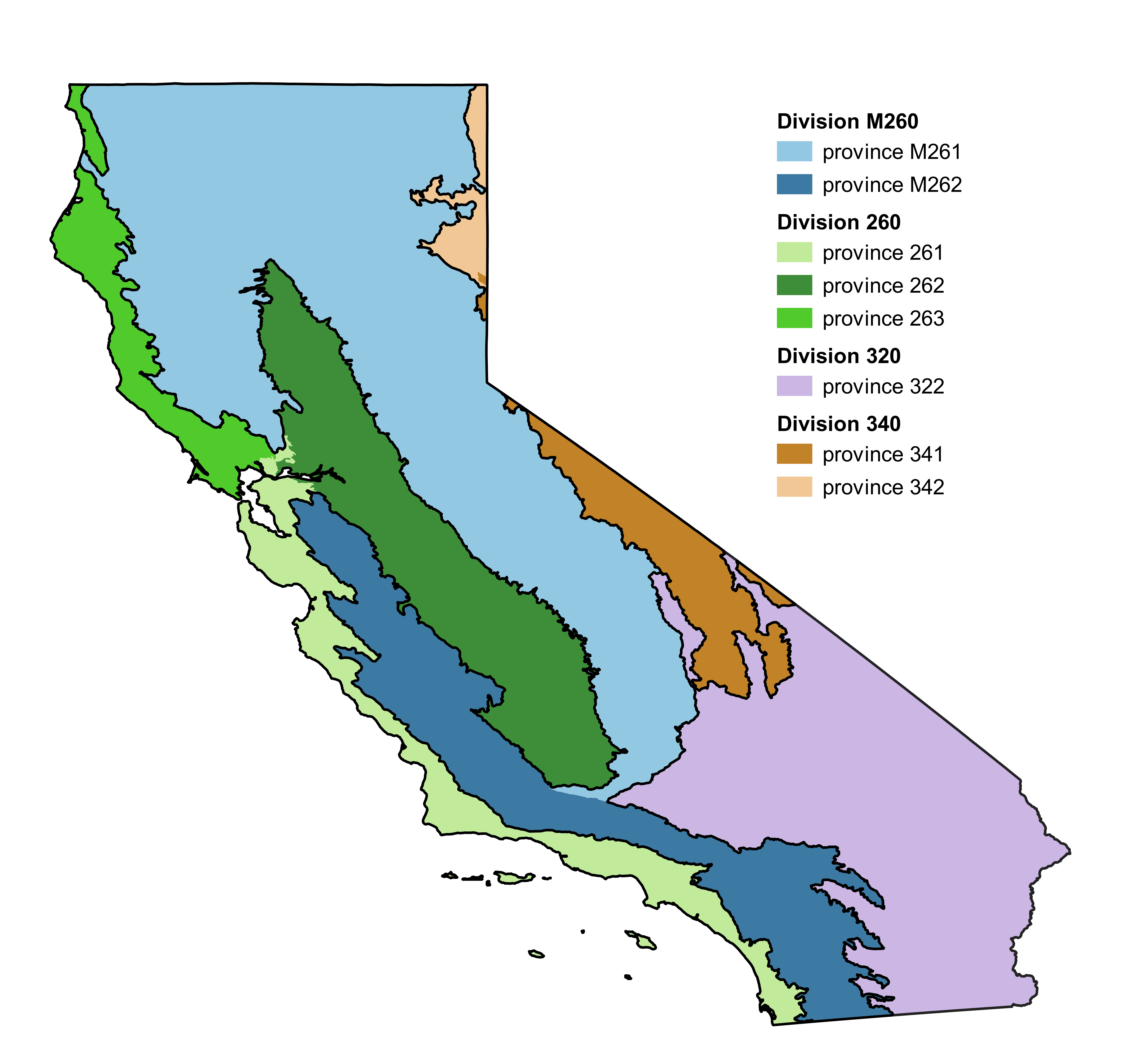
The NSVB framework uses Ecological Divisions. Divisions are further broken down into provinces. You can download the zipped shapefile from HERE to determine the division(s) and province(s) your study site(s) fall into. The provided shapefile covers the entire continental United States.
We also created the map below as a quick help guide specifically for California users (use the shapefile above if your study sites(s) are located outside of California).
| decay class | limbs and branches | top | % bark remaining | sapwood presence and condition | heartwood condition |
|---|---|---|---|---|---|
| 1 | All present | Pointed | 100 | Intact; sound, incipient decay, hard, original color | Sound, hard, original color |
| 2 | Few limbs, no fine branches | May be broken | Variable | Sloughing; advanced decay, fibrous, firm to soft, light brown | Sound at base, incipient decay in outer edge of upper bole, hard, light to reddish brown |
| 3 | Limb studs only | Broken | Variable | Sloughing; fibrous, soft, light to reddish brown | Incipient decay at base, advanced decay throughout upper bole, fibrous, hard to firm, reddish brown |
| 4 | Few or no studs | Broken | Variable | Sloughing; cubical, soft, reddish to dark crown | Advanced decay at base, sloughing from upper bole, fibrous to cubical, soft, dark reddish brown |
| 5 | None | Broken | Less than 20 | Gone | Sloughing, cubical, soft, dark brown, OR fibrous, very soft, dark reddish brown, encased in hardened shell |
Reference: USDA Forest Service. (2019). Forest Inventory and Analysis national core field guide, volume I: Field data collection procedures for phase 2 plots. Version 9.0.
Current SDI is calculated at the plot level for live trees with DBH >= 2.54 cm (1.0 in) as:
\(\sum sph_{i} \left(\frac{dbh_{i}}{25.4}\right)^{1.6}\)
where
Maximum SDI is derived from the 30 × 30 m spatial dataset developed by Chivhenge et al. (2025) for the continental US. We aggregated these estimates by calculating the median maximum SDI within Ecological Subsections (see below for details on subsections). We chose this spatial scale because (1) subsections represent the finest level of the US Forest Service National Hierarchical Framework of Ecological Units (one of the few frameworks that systematically divides the entire continental US into areas with similar geophysical and ecological characteristics) and delineate areas with similar soils, climate, hydrology, and vegetation; and (2) there is substantial uncertainty associated with individual 30 x 30 m estimates. We used the median rather than the mean to reduce the influence of skewed values within subsections. We consulted with Christopher Woodall, a coauthor of Chivhenge et al. (2025), regarding our framework and the associated methodological decisions.
Chivhenge, E., A.R. Weiskittel, C.W. Woodall, A.W. D’Amato, & A. Daigneault. (2025). Geospatial estimation of forest relative density for carbon stewardship decision support across the continental US. Scientific Data, 12, 1728. https://doi.org/10.1038/s41597-025-06012-6
The US Forest Service developed the National Hierarchical Framework
of Ecological Units, which consists of five nested levels: domains,
divisions, provinces, sections, and subsections. The framework was
initially implemented in 2007 and updated in 2025. The NSVB framework
was developed using the 2007 version, whereas the maximum SDI values
used in StandDensity() are based on the updated 2025
version. The spatial boundaries and naming conventions of ecological
units do not align perfectly between the 2007 and 2025 versions.
You can download the Ecosys_EcomapSubsections_2025 shapefile from HERE to determine the subsection(s) your study site(s) fall into.
This suite of functions estimates surface and ground fuel loads (i.e., mass per unit area) from line-intercept transect data. The functions follow the general methodology first described in Stephens (2001):
“Surface and ground fuel loads were calculated by using appropriate equations developed for Sierra Nevada forests (van Wagtendonk et al. 1996, 1998). Coefficients required to calculate all surface and ground fuel loads were arithmetically weighted by the basal area fraction (percentage of total basal area by species) to produce accurate estimates of fuel loads (Jan van Wagtendonk, personal communication, 1999).”
Details on how BerkeleyForestAnalytics calculates
duff/litter, fine, and coarse fuel loads are below. However, note that
in all cases we assume the user collected field data following Brown
(1974) or a similar method in the Sierra Nevada. These
functions should not be used for data collected in a different manner or
region. Additionally, note that to stay consistent with previous
studies, we use both live and dead trees to calculate percent basal area
by species.
All species currently recognized in the surface and ground fuel load functions are listed below.
| common name | scientific name | 4-letter code | FIA code |
|---|---|---|---|
| White fir | Abies concolor | ABCO | 15 |
| California red fir | Abies grandis | ABMA | 20 |
| Incense cedar | Calocedrus decurrens | CADE | 81 |
| Western juniper | Juniperus occidentalis | JUOC | 64 |
| Whitebark pine | Pinus albicaulis | PIAL | 101 |
| Knobcone pine | Pinus attenuata | PIAT | 103 |
| Foxtail pine | Pinus balfourianae | PIBA | 104 |
| Lodgepole pine | Pinus contorta | PICO | 108 |
| Limber pine | Pinus flexilis | PIFL | 113 |
| Jeffrey pine | Pinus jeffreyi | PIJE | 116 |
| Sugar pine | Pinus lambertinana | PILA | 117 |
| Singleleaf pinyon | Pinus monophylla | PIMO1 | 133 |
| Western white pine | Pinus monticola | PIMO2 | 119 |
| Ponderosa pine | Pinus ponderosa | PIPO | 122 |
| Foothill pine | Pinus sabiniana | PISA | 127 |
| Washoe pine | Pinus ponderosa var. washoensis | PIWA | 137 |
| Douglas-fir | Pseudotsuga menziesii | PSME | 202 |
| Giant sequoia | Sequoiadendron giganteum | SEGI | 212 |
| Mountain hemlock | Tsuga mertensiana | TSME | 264 |
| Unknown conifer | NA | UNCO | 299 |
| Unknown hardwood | NA | UNHA | 998 |
| Unknown tree | NA | UNTR | 999 |
Duff and litter (or combined duff/litter) are measured as depths at specific points along a sampling transect. Van Wagtendonk et al. (1998) developed regressions for duff, litter, and combined duff/litter loadings as a function of depth for 19 different Sierra Nevada conifer species:
| common name | scientific name | 4-letter code | FIA code | litter coefficient | duff coefficient | litter/duff coefficient |
|---|---|---|---|---|---|---|
| White fir | Abies concolor | ABCO | 15 | 1.050 | 1.518 | 1.572 |
| California red fir | Abies grandis | ABMA | 20 | 0.530 | 1.727 | 1.722 |
| Incense cedar | Calocedrus decurrens | CADE | 81 | 1.276 | 1.675 | 1.664 |
| Western juniper | Juniperus occidentalis | JUOC | 64 | 0.832 | 1.798 | 1.763 |
| Whitebark pine | Pinus albicaulis | PIAL | 101 | 0.540 | 1.895 | 1.802 |
| Knobcone pine | Pinus attenuata | PIAT | 103 | 0.336 | 1.646 | 1.274 |
| Foxtail pine | Pinus balfourianae | PIBA | 104 | 0.886 | 1.220 | 2.360 |
| Lodgepole pine | Pinus contorta | PICO | 108 | 0.951 | 1.671 | 1.612 |
| Limber pine | Pinus flexilis | PIFL | 113 | 0.889 | 2.337 | 2.255 |
| Jeffrey pine | Pinus jeffreyi | PIJE | 116 | 0.358 | 1.707 | 1.496 |
| Sugar pine | Pinus lambertinana | PILA | 117 | 0.304 | 1.396 | 1.189 |
| Singleleaf pinyon | Pinus monophylla | PIMO1 | 133 | 0.906 | 2.592 | 2.478 |
| Western white pine | Pinus monticola | PIMO2 | 119 | 0.542 | 1.422 | 1.485 |
| Ponderosa pine | Pinus ponderosa | PIPO | 122 | 0.276 | 1.402 | 1.233 |
| Foothill pine | Pinus sabiniana | PISA | 127 | 0.111 | 1.448 | 2.504 |
| Washoe pine | Pinus ponderosa var. washoensis | PIWA | 137 | 0.600 | 1.870 | 1.719 |
| Douglas-fir | Pseudotsuga menziesii | PSME | 202 | 0.864 | 1.319 | 1.295 |
| Giant sequoia | Sequoiadendron giganteum | SEGI | 212 | 0.990 | 1.648 | 1.632 |
| Mountain hemlock | Tsuga mertensiana | TSME | 264 | 1.102 | 1.876 | 1.848 |
| Unknown conifer | NA | UNCO | 299 | 0.363 | 1.75 | 1.624 |
| Unknown hardwood | NA | UNHA | 998 | 0.363 | 1.75 | 1.624 |
| Unknown tree | NA | UNTR | 999 | 0.363 | 1.75 | 1.624 |
Note: UNCO, UNHA, UNTR, and any other species not listed in the table are assigned the “All Species” values provided by van Wagtendonk et al. (1998).
The plot-level fuel load can be calculated using the following equation:
\(F_{p} = \frac{\sum(F_{t})}{n}\)
where
We can calculate \(F_{t}\) using the following equation:
\(F_{t} = d_{t}*coef_{p}\)
where
We can calculate \(coef_{p}\) by averaging together the different species-specific coefficients for each tree species contributing fuel to the plot, weighted by their local prevalence. Specifically, we weight each species’ coefficient by the proportion of total basal area contributed by that species:
\(coef_{p} = \sum((\frac{BA_{sp,p}}{BA_{total,p}})*coef_{sp})\)
where
A note on units: the van Wagtendonk et al. (1998) equations
require depths in cm and output fuel loads in \(kg/m^2\). Any unit conversions (for input
or outputs) must be done by the user.
BerkeleyForestAnalytics does the necessary unit conversions
for you!
Calculating fuel loads represented by transect counts of 1-hour, 10-hour, and 100-hour fuels is more complicated, but follows the same general idea as described for duff and litter above. The plot-level fuel load can be calculated using the following equation:
\(W_{c,p} = \frac{\sum(W_{c,t})}{n}\)
where
We can calculate \(W_{c,t}\) using the equation provided by van Wagtendonk et al. (1996) (modified from Brown (1974)):
\(W_{c,t} = \frac{QMD_{c,p} * SEC_{c,p} * SG_{c,p} * SLP_{t} * k * n_{c,t}}{length_{c,t}}\)
where
Quadratic mean diameter (QMD), secant of acute angle (SEC), and specific gravity (SG)
QMD, SEC, and SG vary by species and timelag class (see tables below with values from van Wagtendonk et al. (1996)). We can calculate \(QMD_{c,p}\) using the following equation:
\(QMD_{c,p} = \sum(\frac{BA_{sp,p}}{BA_{total,p}}*QMD_{c,sp})\)
where
The process is the same for \(SEC_{c,p}\) and \(SG_{c,p}\).
Averaged squared quadratic mean diameter by fuel size class
| common name | scientific name | 4-letter code | FIA code | 1-hour | 10-hour | 100-hour |
|---|---|---|---|---|---|---|
| White fir | Abies concolor | ABCO | 15 | 0.08 | 1.32 | 11.56 |
| California red fir | Abies grandis | ABMA | 20 | 0.10 | 1.32 | 16.24 |
| Incense cedar | Calocedrus decurrens | CADE | 81 | 0.09 | 1.23 | 20.79 |
| Western juniper | Juniperus occidentalis | JUOC | 64 | 0.08 | 1.61 | 13.92 |
| Whitebark pine | Pinus albicaulis | PIAL | 101 | 0.13 | 1.21 | 14.75 |
| Knobcone pine | Pinus attenuata | PIAT | 103 | 0.10 | 1.25 | 9.68 |
| Foxtail pine | Pinus balfourianae | PIBA | 104 | 0.12 | 0.92 | 12.82 |
| Lodgepole pine | Pinus contorta | PICO | 108 | 0.10 | 1.44 | 13.39 |
| Limber pine | Pinus flexilis | PIFL | 113 | 0.21 | 1.28 | 17.72 |
| Jeffrey pine | Pinus jeffreyi | PIJE | 116 | 0.15 | 1.25 | 17.31 |
| Sugar pine | Pinus lambertinana | PILA | 117 | 0.12 | 1.46 | 13.61 |
| Singleleaf pinyon | Pinus monophylla | PIMO1 | 133 | 0.09 | 1.41 | 11.56 |
| Western white pine | Pinus monticola | PIMO2 | 119 | 0.08 | 0.79 | 9.92 |
| Ponderosa pine | Pinus ponderosa | PIPO | 122 | 0.23 | 1.56 | 19.36 |
| Foothill pine | Pinus sabiniana | PISA | 127 | 0.14 | 0.94 | 12.91 |
| Washoe pine | Pinus ponderosa var. washoensis | PIWA | 137 | 0.22 | 1.37 | 13.47 |
| Douglas-fir | Pseudotsuga menziesii | PSME | 202 | 0.06 | 1.37 | 12.04 |
| Giant sequoia | Sequoiadendron giganteum | SEGI | 212 | 0.14 | 1.28 | 17.06 |
| Mountain hemlock | Tsuga mertensiana | TSME | 264 | 0.05 | 1.46 | 13.61 |
| Unknown conifer | NA | UNCO | 299 | 0.12 | 1.28 | 14.52 |
| Unknown hardwood | NA | UNHA | 998 | 0.12 | 1.28 | 14.52 |
| Unknown tree | NA | UNTR | 999 | 0.12 | 1.28 | 14.52 |
Average secant of acute angles of inclinations of nonhorizontal particles by fuel size class
| common name | scientific name | 4-letter code | FIA code | 1-hour | 10-hour | 100-hour | 1000-hour |
|---|---|---|---|---|---|---|---|
| White fir | Abies concolor | ABCO | 15 | 1.03 | 1.02 | 1.02 | 1.01 |
| California red fir | Abies grandis | ABMA | 20 | 1.03 | 1.02 | 1.01 | 1.00 |
| Incense cedar | Calocedrus decurrens | CADE | 81 | 1.02 | 1.02 | 1.03 | 1.06 |
| Western juniper | Juniperus occidentalis | JUOC | 64 | 1.03 | 1.04 | 1.04 | 1.04 |
| Whitebark pine | Pinus albicaulis | PIAL | 101 | 1.02 | 1.02 | 1.02 | 1.02 |
| Knobcone pine | Pinus attenuata | PIAT | 103 | 1.03 | 1.02 | 1.00 | 1.02 |
| Foxtail pine | Pinus balfourianae | PIBA | 104 | 1.02 | 1.02 | 1.01 | 1.02 |
| Lodgepole pine | Pinus contorta | PICO | 108 | 1.02 | 1.02 | 1.01 | 1.05 |
| Limber pine | Pinus flexilis | PIFL | 113 | 1.02 | 1.02 | 1.01 | 1.01 |
| Jeffrey pine | Pinus jeffreyi | PIJE | 116 | 1.03 | 1.03 | 1.04 | 1.05 |
| Sugar pine | Pinus lambertinana | PILA | 117 | 1.04 | 1.04 | 1.03 | 1.03 |
| Singleleaf pinyon | Pinus monophylla | PIMO1 | 133 | 1.02 | 1.01 | 1.01 | 1.05 |
| Western white pine | Pinus monticola | PIMO2 | 119 | 1.03 | 1.02 | 1.06 | 1.02 |
| Ponderosa pine | Pinus ponderosa | PIPO | 122 | 1.02 | 1.03 | 1.02 | 1.01 |
| Foothill pine | Pinus sabiniana | PISA | 127 | 1.05 | 1.03 | 1.02 | 1.02 |
| Washoe pine | Pinus ponderosa var. washoensis | PIWA | 137 | 1.02 | 1.02 | 1.01 | 1.05 |
| Douglas-fir | Pseudotsuga menziesii | PSME | 202 | 1.03 | 1.02 | 1.03 | 1.04 |
| Giant sequoia | Sequoiadendron giganteum | SEGI | 212 | 1.02 | 1.02 | 1.02 | 1.01 |
| Mountain hemlock | Tsuga mertensiana | TSME | 264 | 1.04 | 1.02 | 1.02 | 1.00 |
| Unknown conifer | NA | UNCO | 299 | 1.03 | 1.02 | 1.02 | 1.02 |
| Unknown hardwood | NA | UNHA | 998 | 1.03 | 1.02 | 1.02 | 1.02 |
| Unknown tree | NA | UNTR | 999 | 1.03 | 1.02 | 1.02 | 1.02 |
Average specific gravity by fuel size class
| common name | scientific name | 4-letter code | FIA code | 1-hour | 10-hour | 100-hour | 1000-hour sound | 1000-hour rotten |
|---|---|---|---|---|---|---|---|---|
| White fir | Abies concolor | ABCO | 15 | 0.53 | 0.54 | 0.57 | 0.32 | 0.36 |
| California red fir | Abies grandis | ABMA | 20 | 0.57 | 0.56 | 0.47 | 0.38 | 0.36 |
| Incense cedar | Calocedrus decurrens | CADE | 81 | 0.59 | 0.54 | 0.55 | 0.41 | 0.36 |
| Western juniper | Juniperus occidentalis | JUOC | 64 | 0.67 | 0.65 | 0.62 | 0.47 | 0.36 |
| Whitebark pine | Pinus albicaulis | PIAL | 101 | 0.55 | 0.49 | 0.48 | 0.42 | 0.36 |
| Knobcone pine | Pinus attenuata | PIAT | 103 | 0.59 | 0.55 | 0.39 | 0.47 | 0.36 |
| Foxtail pine | Pinus balfourianae | PIBA | 104 | 0.59 | 0.61 | 0.53 | 0.47 | 0.36 |
| Lodgepole pine | Pinus contorta | PICO | 108 | 0.53 | 0.48 | 0.54 | 0.58 | 0.36 |
| Limber pine | Pinus flexilis | PIFL | 113 | 0.57 | 0.57 | 0.54 | 0.63 | 0.36 |
| Jeffrey pine | Pinus jeffreyi | PIJE | 116 | 0.53 | 0.55 | 0.55 | 0.47 | 0.36 |
| Sugar pine | Pinus lambertinana | PILA | 117 | 0.59 | 0.59 | 0.52 | 0.43 | 0.36 |
| Singleleaf pinyon | Pinus monophylla | PIMO1 | 133 | 0.65 | 0.64 | 0.53 | 0.47 | 0.36 |
| Western white pine | Pinus monticola | PIMO2 | 119 | 0.56 | 0.56 | 0.49 | 0.47 | 0.36 |
| Ponderosa pine | Pinus ponderosa | PIPO | 122 | 0.55 | 0.56 | 0.48 | 0.40 | 0.36 |
| Foothill pine | Pinus sabiniana | PISA | 127 | 0.64 | 0.61 | 0.43 | 0.47 | 0.36 |
| Washoe pine | Pinus ponderosa var. washoensis | PIWA | 137 | 0.53 | 0.52 | 0.44 | 0.35 | 0.36 |
| Douglas-fir | Pseudotsuga menziesii | PSME | 202 | 0.60 | 0.61 | 0.59 | 0.35 | 0.36 |
| Giant sequoia | Sequoiadendron giganteum | SEGI | 212 | 0.57 | 0.57 | 0.56 | 0.54 | 0.36 |
| Mountain hemlock | Tsuga mertensiana | TSME | 264 | 0.67 | 0.65 | 0.62 | 0.66 | 0.36 |
| Unknown conifer | NA | UNCO | 299 | 0.58 | 0.57 | 0.53 | 0.47 | 0.36 |
| Unknown hardwood | NA | UNHA | 998 | 0.58 | 0.57 | 0.53 | 0.47 | 0.36 |
| Unknown tree | NA | UNTR | 999 | 0.58 | 0.57 | 0.53 | 0.47 | 0.36 |
Notes for the above tables:
Slope correction factor (SLP)
We can calculate \(SLP_{t}\) using the equation provided by Brown (1974):
\(SLP_{t} = \sqrt{1 + (\frac{slope_{t}}{100})^2}\)
where
Equation constant k
Equation constant K for input and output units. These values are from van Wagner (1982) and are used in van Wagtendonk et al. (1996).
| fuel diameter | transect length | mass per unit area | k |
|---|---|---|---|
| cm | m | \(kg/m^2\) | 0.1234 |
| cm | m | metric tons/ha | 1.234 |
| in | ft | \(lb/ft^2\) | 0.5348 |
| in | ft | US tons/ac | 11.65 |
Calculating loads for 1000-hour fuels is just a special case of the equations given above for 1-100 hour fuels. The difference is that instead of counted intercepts and an average squared quadratic mean diameter, we have the actual sum of squared diameters from the field data. The plot-level fuel load can be calculated using the following equation:
\(W_{1000h,p} = \frac{\sum(W_{1000h,t})}{n}\)
where
We can calculate \(W_{1000h,t}\) using the equation provided by Brown (1974):
\(W_{1000h,t} = \frac{\sum(d^2_{t}) * SEC_{1000h,p} * SG_{1000h,s,p} * SLP_{t} * k}{length_{1000h,t}}\)
where
For \(SEC_{1000h,p}\), \(SG_{1000h,s,p}\), \(SLP_{t}\), and \(k\) see fine fuel loads documentation above - the same concepts are applied here.
In the above calculations, we used the slope correction factor from Brown (1974) for converting mass per unit area on a slope basis to a horizontal basis. However, for further compilation (e.g., to the stratum or site level), we should “weight estimates by the length of the line transect actually sampled” (Marshall et al. 2000).
Marshall et al. (2000) describes the importance of obtaining horizontal transect length:
“To obtain an unbiased estimate, the horizontal transect length must be known. Preferably, all transects should be corrected for slope in the field so that all transects are of equal horizontal length. This simplifies the compilation and subsequent analyses.”
“If unequal line transect lengths exisit within a sample an unbiased estimate of the variance of any CWD estimate is no longer guaranteed. It is usually best to weight the estimate, giving values from longer line transects proportionally more weight than those from shorter transects.”
We can calculate the total horizontal length of transect sampled at a specific plot using the following equation:
\(SCLength_{c,p} = \sum(SCLength_{c,t})\)
where
Why are we calculating horizontal length at the plot-level? Transects can be different shapes, most often single lines, stars, or triangles (see diagram on pg. 4 of Marshall et al. 2000). “Each line transect, irrespective of shape, represents a single sampling unit… The shape and length of a line transect will vary depending on the protocol employed. For example, a triangle with three 30-m lines (i.e., a 90-m transect) is often used for determining fuel load prior to a prescribed burn…” (Marshall et al. 2000). We often use “transect” to describe an individual line (e.g., one of the the 30-m lines) rather than to describe the sampling unit (e.g., the 90-m transect). It can be helpful to remember that “… the sampling points are located, not the line transect. The sampling point represents a designated position on the line transect. In most cases the sampling point is the end point of the line transect, and is where piece measurements are initiated. Once a sample point is located, the line transect is installed following a specific routine” (Marshall et al. 2000). In many forestry scenarios, the sampling point will be plot center.
We can calculate \(SCLength_{c,t}\) using the following equation:
\(SCLength_{c,t} = cos(SlopeDeg_t)*Length_{c,t}\)
where
We can calculate \(SlopeDeg_t\) using the following equation:
\(SlopeDeg_t = tan^{-1}(\frac{SlopePerc_t}{100})\)
where
References:
Brown, J.K. (1974). Handbook for inventorying downed woody material. General Technical Report INT-16. USDA Forest Service, Intermountain Forest and Range Experiment Station, Ogden, UT. https://research.fs.usda.gov/treesearch/28647
Marshall, P.L., Davis, G., & LeMay, V.M. (2000). Using line intersect sampling for coarse woody debris. Forest Research Technical Report TR-003. British Columbia Ministry of Forests, Vancouver Forest Region, Nanaimo, BC.
Stephens, S.L. (2001). Fire history differences in adjacent Jeffrey pine and upper montane forests in the eastern Sierra Nevada. International Journal of Wildland Fire, 10(2), 161–167. https://doi.org/10.1071/WF01008
Van Wagner, C.E. (1982). Practical aspects of the line intersect method. Information Report PI-X-12. Petawawa National Forestry Institute, Canadian Forestry Service, Chalk River, Ontario. https://ostrnrcan-dostrncan.canada.ca/entities/publication/d1289126-5f22-421f-9805-519a326d83ca
van Wagtendonk, J.W., Benedict, J.M., & Sydoriak, W.M. (1996). Physical properties of woody fuel particles of Sierra Nevada conifers. International Journal of Wildland Fire, 6(3), 117–123. https://doi.org/10.1071/WF9960117
van Wagtendonk, J.W., Benedict, J.M. & Sydoriak, W.M. (1998). Fuel bed characteristics of Sierra Nevada conifers. Western Journal of Applied Forestry, 13(3), 73–84. https://doi.org/10.1093/wjaf/13.3.73
General definition of finite population correction factor (FPC):
\(\frac{N-n}{N}\)
where
FPC is a modifier used on the standard error:
\(s_{\bar{y}} = \sqrt{\frac{s_y^2}{n}*\frac{N-n}{N}}\)
“[The] fpc will always be a number between 0 and 1. To understand the purpose of the fpc, first look at the most intensive sampling situation. If all sampling units in the population were measured (that is, n = N, a 100% sample), then the sample mean would be the population mean (that is, everything in the population was measured, so the true population mean is known). Therefore, the estimate of the population mean has no variability, and since the fpc equals zero, the variance of the sample mean… is also zero. [Without the fpc], the variance estimate of the mean would not be zero when all sampling units are measured, which would be illogical… it seems logical that if n is almost as big as N, the resulting means of different samples of size n will have less variability than they would if n were smaller relative to N. This is the desirable logical property that the fpc gives \(s_{\bar{y}}\)” (Shiver and Borders 1996, pg. 33).
When to use FPC:
“The units may be selected with or without replacement. If selection is with replacement, each unit is allowed to appear in the sample as often as it is selected. In sampling without replacement, a particular unit is allowed to appear in the sample only once. Most forest sampling is without replacement… the procedure for computing standard errors depends on whether sampling was with or without replacement… [The fpc] is used when units are selected without replacement. If units are selected with replacement, the fpc is omitted… Even when sampling is without replacement, the sampling fraction (n/N) may be extremely small, making the fpc very close to unity. If n/N is less than 0.05, the fpc is commonly ignored and the standard error computed from the shortened formula” (Freese 1962, pg. 21-23).
In summary, you only need to use the FPC if:
Note: the recommendation to ignore the FPC when the sampling fraction is less than 0.05 is common throughout forest sampling textbooks. We recommend BFA users follow this accepted 5% rule.
An example of how to get N:
References:
Freese, F. (1962). Elementary forest sampling. Agriculture Handbook No. 232. USDA Forest Service, Southern Forest Experiment Station. https://www.govinfo.gov/content/pkg/GOVPUB-A-PURL-gpo21243/pdf/GOVPUB-A-PURL-gpo21243.pdf
Shiver, B.D., & Borders, B.E. (1996). Sampling techniques for forest resource inventory. J. Wiley, New York, New York, USA.
A general note on data compilation: If you have a stratified random sampling design, you must calculate stratum values before calculating overall values. Similarly, for the Fire and Fire Surrogate design, you must calculate compartment values before calculating overall values.
Simple random sampling
Mean:
\(\bar{y} = \frac{\sum(y_i)}{n}\)
Standard error:
\(s_y^2 = \frac{\sum(y_i^2) - \frac{(\sum(y_i))^2}{n}}{n-1}\)
without FPC, \(s_{\bar{y}} = \sqrt{\frac{s_y^2}{n}}\)
with FPC, \(s_{\bar{y}} = \sqrt{\frac{s_y^2}{n}*\frac{N-n}{N}}\)
Definitions:
Stratified random sampling
Stratum values ———————————
Mean:
\(\bar{y_h} = \frac{\sum(y_{h_i})}{n_h}\)
Standard error:
\(s_{y_h}^2 = \frac{\sum(y_{h_i}^2) - \frac{(\sum(y_{h_i}))^2}{n_h}}{n_h-1}\)
without FPC, \(s_{\bar{y_h}} = \sqrt{\frac{s_{y_h}^2}{n_h}}\)
with FPC, \(s_{\bar{y_h}} = \sqrt{\frac{s_{y_h}^2}{n_h}*\frac{N_h-n_h}{N_h}}\)
Definitions:
Overall values ———————————-
Mean:
\(\bar{y} = \sum(\bar{y_h} * W_h)\)
Standard error:
\(s_{\bar{y}} = \sqrt{\sum(s_{\bar{y_h}}^2 * W_h^2)}\)
Definitions:
Fire and Fire Surrogate
Compartment values ——————————-
Mean:
\(\bar{y_c} = \frac{\sum(y_{c_i})}{n_c}\)
Standard error:
\(s_{y_c}^2 = \frac{\sum(y_{c_i}^2) - \frac{(\sum(y_{c_i}))^2}{n_c}}{n_c-1}\)
without FPC, \(s_{\bar{y_c}} = \sqrt{\frac{s_{y_c}^2}{n_c}}\)
with FPC, \(s_{\bar{y_c}} = \sqrt{\frac{s_{y_c}^2}{n_c}*\frac{N_c-n_c}{N_c}}\)
Definitions:
Overall values ———————————–
Mean:
\(\bar{y} = \frac{\sum(y_c)}{n}\)
Standard error:
\(s_y^2 = \frac{\sum(y_c^2) - \frac{(\sum(y_c))^2}{n}}{n-1}\)
\(s_{\bar{y}} = \sqrt{\frac{s_y^2}{n}}\)
Definitions:
A general note on data compilation: If you have a stratified random sampling design, you must calculate stratum values before calculating overall values. Similarly, for the Fire and Fire Surrogate design, you must calculate compartment values before calculating overall values.
See Slope-corrected transect length section above for additional background information. The equations below are applicable for summarizing 1-hour, 10-hour, 100-hour, and 1000-hour fuel loads. For other surface and ground fuel load combinations (e.g., 1-hour + 10-hour + 100-hour + litter), create the necessary columns and use the general equations provided above (weighting the estimates by the length of the line transect is not applicable in the same way for these combined fuel loads).
Simple random sampling
Weighted mean:
\(\bar{y} = \frac{\sum(w_i*y_i)}{n}\)
Weighted standard error:
without FPC, \(s_{\bar{y}} = \sqrt{\frac{\sum(w_i*(y_i-\bar{y})^2)}{n*(n-1)}}\)
with FPC, \(s_{\bar{y}} = \sqrt{\frac{\sum(w_i*(y_i-\bar{y})^2)}{n*(n-1)}*\frac{N-n}{N}}\)
Definitions:
Stratified random sampling
Stratum values ———————————
Weighted mean:
\(\bar{y_h} = \frac{\sum(w_{h_i}*y_{h_i})}{n_h}\)
Weighted standard error:
\(s_{y_h}^2 = \frac{\sum(w_{h_i}*(y_{h_i}-\bar{y_h})^2)}{n_h-1}\)
without FPC, \(s_{\bar{y_h}} = \sqrt{\frac{s_{y_h}^2}{n_h}}\)
with FPC, \(s_{\bar{y_h}} = \sqrt{\frac{s_{y_h}^2}{n_h}*\frac{N_h-n_h}{N_h}}\)
Definitions:
Overall values ———————————-
Mean:
\(\bar{y} = \sum(\bar{y_h} * W_h)\)
Standard error:
\(s_{\bar{y}} = \sqrt{\sum(s_{\bar{y_h}}^2 * W_h^2)}\)
Definitions:
Fire and Fire Surrogate
Compartment values ——————————
Weighted mean:
\(\bar{y_c} = \frac{\sum(w_{c_i}*y_{c_i})}{n_c}\)
Weighted standard error:
\(s_{y_c}^2 = \frac{\sum(w_{c_i}*(y_{c_i}-\bar{y_c})^2)}{n_c-1}\)
without FPC, \(s_{\bar{y_c}} = \sqrt{\frac{s_{y_c}^2}{n_c}}\)
with FPC, \(s_{\bar{y_c}} = \sqrt{\frac{s_{y_c}^2}{n_c}*\frac{N_c-n_c}{N_c}}\)
Definitions:
Overall values ———————————-
Mean:
\(\bar{y} = \frac{\sum(y_c)}{n}\)
Standard error:
\(s_y^2 = \frac{\sum(y_c^2) - \frac{(\sum(y_c))^2}{n}}{n-1}\)
\(s_{\bar{y}} = \sqrt{\frac{s_y^2}{n}}\)
Definitions:
Kea Rutherford maintains BerkeleyForestAnalytics. Please
reach out if you find a bug.
Contact email: krutherford@berkeley.edu