![]()
![]()
Package: cbbinom
0.2.0
Author: Xiurui Zhu
Modified: 2024-09-18 23:27:13
Compiled: 2024-10-16 23:21:42
The goal of cbbinom is to implement continuous
beta-binomial distribution.
You can install the released version of cbbinom from CRAN with:
install.packages("cbbinom")Alternatively, you can install the developmental version of
cbbinom from github
with:
remotes::install_github("zhuxr11/cbbinom")The continuous beta-binomial distribution spreads the standard
probability mass of beta-binomial distribution at x to an
interval [x, x + 1] in a continuous manner. This can be
validated via the following plot, where we can see that the cumulative
distribution function (CDF) of the continuous beta-binomial distribution
at x + 1 equals to that of the beta-binomial distribution
at x.
library(cbbinom)# The continuous beta-binomial CDF, shift by -1
cbbinom_plot_x <- seq(-1, 10, 0.01)
cbbinom_plot_y <- pcbbinom(
q = cbbinom_plot_x,
size = 10,
alpha = 2,
beta = 4,
ncp = -1
)
# The beta-binomial CDF
bbinom_plot_x <- seq(0L, 10L, 1L)
bbinom_plot_y <- extraDistr::pbbinom(
q = bbinom_plot_x,
size = 10L,
alpha = 2,
beta = 4
)
ggplot2::ggplot(mapping = ggplot2::aes(x = x, y = y)) +
ggplot2::geom_bar(
data = data.frame(
x = bbinom_plot_x,
y = bbinom_plot_y
),
stat = "identity"
) +
ggplot2::geom_point(
data = data.frame(
x = cbbinom_plot_x,
y = cbbinom_plot_y
)
) +
ggplot2::scale_x_continuous(
n.breaks = diff(range(cbbinom_plot_x))
) +
ggplot2::theme_bw() +
ggplot2::labs(y = "CDF(x)")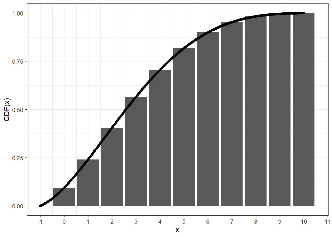
However, the central density at x + 1/2 of the
continuous beta-binomial distribution may not equal to the corresponding
probability mass at x, especially around the summit and to
the right (since alpha < beta).
# The continuous beta-binomial CDF, shift by -1/2
cbbinom_plot_x_d <- seq(-1/2, 10 + 1/2, 0.01)
cbbinom_plot_y_d <- dcbbinom(
  x = cbbinom_plot_x_d,
  size = 10,
  alpha = 2,
  beta = 4,
  ncp = -1/2
)
# The beta-binomial CDF
bbinom_plot_x <- seq(0L, 10L, 1L)
bbinom_plot_y_d <- extraDistr::dbbinom(
  x = bbinom_plot_x,
  size = 10L,
  alpha = 2,
  beta = 4
)
ggplot2::ggplot(mapping = ggplot2::aes(x = x, y = y)) +
  ggplot2::geom_bar(
    data = data.frame(
      x = bbinom_plot_x,
      y = bbinom_plot_y_d
    ),
    stat = "identity"
  ) +
  ggplot2::geom_point(
    data = data.frame(
      x = cbbinom_plot_x_d,
      y = cbbinom_plot_y_d
    )
  ) +
  ggplot2::scale_x_continuous(
    n.breaks = diff(range(bbinom_plot_x))
  ) +
  ggplot2::theme_bw() +
  ggplot2::labs(y = "PDF(x)")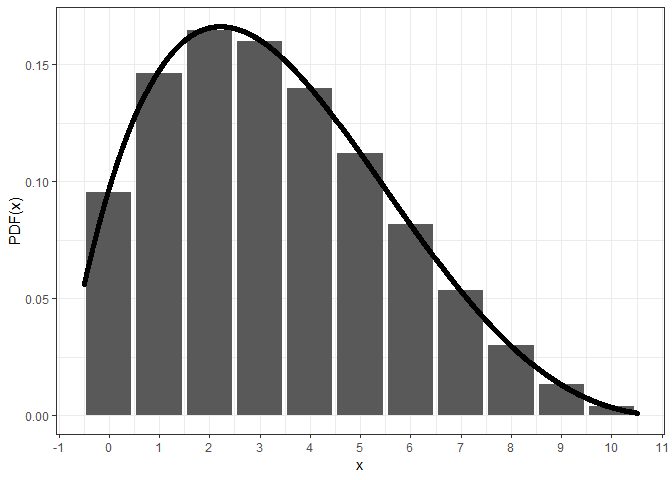
For larger sizes, you may need higher precision than double for accuracy, at the cost of computational speed.
cbbinom_plot_prec_x_p <- seq(0, 41, 0.1)
# Compute CDF at default (double) precision level
system.time(pcbbinom_plot_prec0_y <- pcbbinom(
  q = cbbinom_plot_prec_x_p,
  size = 40,
  alpha = 2,
  beta = 4,
  prec = NULL
))
#>    user  system elapsed
#> 0.03 0.00 0.03ggplot2::ggplot(data = data.frame(x = cbbinom_plot_prec_x_p,
y = pcbbinom_plot_prec0_y),
mapping = ggplot2::aes(x = x, y = y)) +
ggplot2::geom_point() +
ggplot2::theme_bw() +
ggplot2::labs(y = "CDF(x)")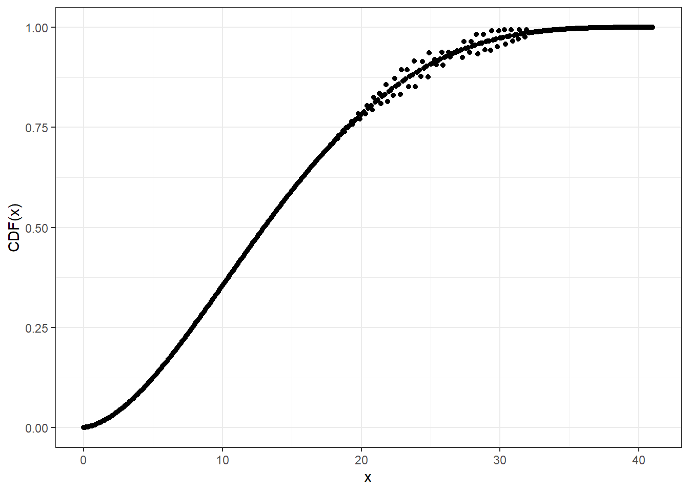
# Compute CDF at precision level 20
system.time(pcbbinom_plot_prec20_y <- pcbbinom(
  q = cbbinom_plot_prec_x_p,
  size = 40,
  alpha = 2,
  beta = 4,
  prec = 20L
))
#>    user  system elapsed
#> 1.57 0.00 1.59ggplot2::ggplot(data = data.frame(x = cbbinom_plot_prec_x_p,
y = pcbbinom_plot_prec20_y),
mapping = ggplot2::aes(x = x, y = y)) +
ggplot2::geom_point() +
ggplot2::theme_bw() +
ggplot2::labs(y = "CDF(x)")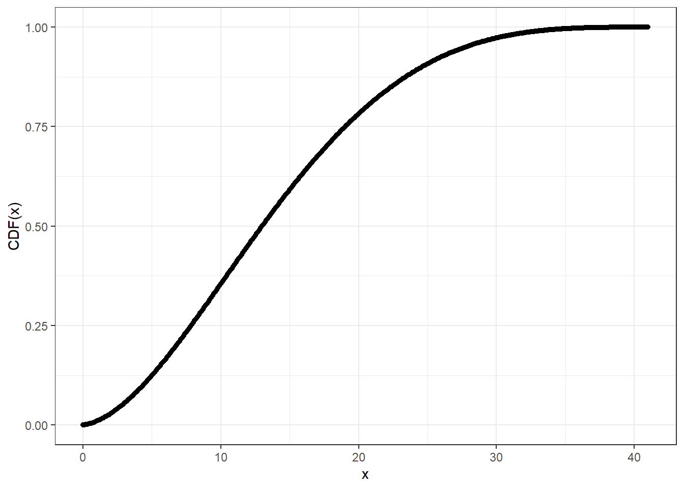
As the probability distributions in stats package,
cbbinom provides a full set of density, distribution
function, quantile function and random generation for the continuous
beta-binomial distribution.
# Density function
dcbbinom(x = 5, size = 10, alpha = 2, beta = 4)
#> [1] 0.12669
# Distribution function
(test_val <- pcbbinom(q = 5, size = 10, alpha = 2, beta = 4))
#> [1] 0.7062937# Quantile function
qcbbinom(p = test_val, size = 10, alpha = 2, beta = 4)
#> [1] 5# Random generation
set.seed(1111L)
rcbbinom(n = 10L, size = 10, alpha = 2, beta = 4)
#> [1] 3.359039 3.038286 7.110936 1.311321 5.264688 8.709005 6.720415 1.164210
#> [9] 3.868370 1.332590These functions are also available in Rcpp as
cbbinom::cpp_*cbbinom(), when using
[[Rcpp::depends(cbbinom)]] and
#include <cbbinom.h>.
For mathematical details, please check the details section of
?cbbinom.
Rcpp
implementation of stats::uniroot()As a bonus, cbbinom also exports an Rcpp
implementation of stats::uniroot() function, which may come
in handy to solve equations, especially the monotonic ones used in
quantile functions. Here is an example to calculate qnorm
from pnorm in Rcpp.
#include <iostream>
#include "cbbinom.h"
using namespace cbbinom;

// Define a functor as pnorm() - p
class PnormEqn: public UnirootEqn
{
private:
  double mu;
  double sd;
  double p;
public:
  PnormEqn(const double mu_, const double sd_, const double p_):
    mu(mu_), sd(sd_), p(p_) {}
  double operator () (const double& x) const override {
    return R::pnorm(x, this->mu, this->sd, true, false) - this->p;
  }
};

// Compute quantiles
int main() {
  double p = 0.975;  // Quantile
  PnormEqn eqn_obj(0.0, 1.0, 0.975);
  double tol = 1e-6;
  int max_iter = 10000;
  double q = cbbinom::cpp_uniroot(-1000.0, 1000.0, -p, 1.0 - p, &eqn_obj, &tol, &max_iter);
  std::cout << "Quantile at " << p << "is: " << q << std::endl;
  return 0;
}