

regMR provides a comprehensive framework for fitting regularized
finite mixture regression models via an MM algorithm. The sparse group
lasso (sgl) penalty is applied to parameter updates within the MM
algorithm for variable selection with respect to groups and covariates.
The package provides multiple functions for estimation and allows users
to fit models over different lambda-alpha sgl penalties and group
counts. There are four families of finite mixture regression models able
to be fit: Gaussian, Poisson, Binomial, and Gamma. These are specified
using the family argument in the three main functions the
package contains, FMRM(), MM_Grid(), and
MM(). The models can also be selected using different
information criteria including the default Bayesian Information
Criterion (BIC), group-structured Extended BIC (gEBIC), Akaike
Information Criterion (AIC), and Integrated Classification Likelihood
(ICL) Criterion. See the documentation for more information regarding
how the arguments are specified.
This readme file provides a brief and basic example of how to use the
regMR package. It walks through generating clustered data to which a
finite Gaussian mixture regression model is fit, applying
FMRM() to carry out that procedure over different
lambda-alpha sgl penalties and group counts, and applying the plotting
and summary methods/functions to the model to get the most use out of
the package.
You can install the development version of regMR from GitHub with:
# install.packages("devtools")
library(devtools)
install_github("vjoshy/regMR")
You can install the released version of regMR from CRAN using:
install.packages("regMR")To generate the clustered data to fit using regMR, we require the
package mvtnorm to be installed. More information on mvtnorm can be
found here: https://CRAN.R-project.org/package=mvtnorm. After
setting the seed to ensure reproducibility of the data, initializing the
simulation parameters (number of samples (n), covariates
(p), mixture components (G), and the
correlation constant (rho)), and defining the true
parameters for the clusters, we can begin to construct the multivariate
normal data (X) and generate the response
(y).
X: To generate X, the correlation matrix
must first be initialized. This is done using the following structure:
\(\Sigma = \{\rho^{|j - k|}\}^p_{j, k =
1}\). Then, with mean 0 and the aforementioned correlation
structure, X (a matrix of size n x p) is generated using
the rmvnorm() function from mvtnorm.
y: To generate y, the group
responsibilities and mean vector must be initialized. For the group
responsibilities, we use the rmultinom() function coupled
with the \(\pi\) vector. For the mean
vector, we calculate \(\beta_0 + \sum^p_{j =
1}x_{ij}\beta_{gj}\), where i goes from 1 to n and g is the group
that the \(i^{th}\) observation belongs
to. Then, using the mean vector and the true standard deviations,
y (a response vector of length n) is generated with
rnorm().
# install.packages("mvtnorm")
library(mvtnorm)

set.seed(2025)

# ----Simulate data----
n <- 500   # total samples
p <- 6     # number of covariates
G <- 3     # number of mixture components
rho = 0.2  # correlation

# ----True parameters for 3 clusters----
betas <- matrix(c(
  1,  2, -1,  0.5, 0, 0, 0,  # component 1
  5, -2,  1,  0, 0, 0, 0,  # component 2
  -3, 0,  2, 0, 0, 0, 0     # component 3
), nrow = G, byrow = TRUE) / 2
pis <- c(0.4, 0.4, 0.2)
sigmas <- c(0.5, 0.4, 0.3)

# ----Generate correlation matrix----
cor_mat <- outer(1:p, 1:p, function(i, j) rho^abs(i - j))
Sigma <- cor_mat

# ----Simulate design matrix X (n × p)----
X <- mvtnorm::rmvnorm(n, mean = rep(0, p), sigma = Sigma)

# ----Generate responsibilities----
z <- rmultinom(n, size = 1, prob = pis)
groups <- apply(z, 2, which.max)

# ----b0 + b1x1 + b2x2 + ... + bkxp----
mu_vec <- rowSums(cbind(1, X) * betas[groups, ])

# ----Simulate response y----
y <- rnorm(n, mean = mu_vec, sd = sigmas[groups])We call FMRM() with family = gaussian() and
information_criteria = "bic" to fit a finite Gaussian
mixture regression model to the data. FMRM() fits
regularized finite mixture regression models via the MM algorithm over a
range of lambda-alpha sgl penalties and group counts. The maximum group
count to be tested is specified in the function below as
G = 4. The function chooses the model with the lowest
information criteria value as specified by the user, which in this case
will be BIC.
# ----Load the regMR package----
library(regMR)
#>
#> ── regMR ───────────────────────────────
#> Version: 0.0.0.9000
#> Type ?regMR for help
#> ────────────────────────────────────────

# ----Fit model----
fit <- FMRM(x = X, y = y, G = 4, family = gaussian(),
            information_criteria = "bic", parallel = TRUE)
#>
#> -- g = 2 --
#> ================================================================================
#>
#>  selected model for g = 2
#>
#>  lambda = 26.32 || alpha = 1 ||  BIC  = 1890.43
#>
#>  Components     1      2
#>  Pi           0.287  0.713
#>  Sigma        0.340  1.306
#>
#>  Beta (Regression Parameters)
#>   Components     1      2
#>   Intercept   -1.503  1.861
#>   Beta 1       0.030 -0.271
#>   Beta 2       0.965  0.321
#>   Beta 3       0.009 -0.000
#>   Beta 4       0.000 -0.000
#>   Beta 5       0.046 -0.000
#>   Beta 6       0.000 -0.000
#>
#>
#> -- g = 3 --
#> ================================================================================
#>
#>  selected model for g = 3
#>
#>  lambda = 54.36 || alpha = 1 ||  BIC  = 1428.6
#>
#>  Components     1      2      3
#>  Pi           0.237  0.335  0.428
#>  Sigma        0.279  0.459  0.384
#>
#>  Beta (Regression Parameters)
#>   Components     1      2      3
#>   Intercept   -1.513  0.502  2.543
#>   Beta 1       0.040  0.984 -1.002
#>   Beta 2       0.990 -0.468  0.492
#>   Beta 3      -0.000  0.179  0.000
#>   Beta 4       0.000  0.000 -0.000
#>   Beta 5       0.029 -0.000 -0.000
#>   Beta 6      -0.000 -0.000 -0.031
#>
#>
#> -- g = 4 --
#> ================================================================================
#>
#>  selected model for g = 4
#>
#>  lambda = 66.04 || alpha = 0.9 ||  BIC  = 1469.17
#>
#>  Components     1      2      3      4
#>  Pi           0.239  0.323  0.025  0.413
#>  Sigma        0.281  0.450  0.021  0.366
#>
#>  Beta (Regression Parameters)
#>   Components     1      2      3      4
#>   Intercept   -1.515  0.476  2.226  2.554
#>   Beta 1       0.043  0.945  0.328 -1.005
#>   Beta 2       0.983 -0.409  0.017  0.481
#>   Beta 3      -0.000  0.129 -0.019  0.000
#>   Beta 4       0.000  0.008  0.001 -0.000
#>   Beta 5       0.028  0.000  0.042 -0.000
#>   Beta 6      -0.000 -0.000 -0.733 -0.023
#>
#> --------------------------------------------------------------------------------
#>
#>  overall model chosen ->
#>
#>  G = 3
#>
#>  lambda = 54.36 || alpha = 1 || log-likelihood = -661.47 ||  BIC  = 1428.6 || MSE = 0.12
#>
#>  Components     1      2      3
#>  Pi           0.237  0.335  0.428
#>  Sigma        0.279  0.459  0.384
#>
#>  Beta (Regression Parameters)
#>   Components     1      2      3
#>   Intercept   -1.513  0.502  2.543
#>   Beta 1       0.040  0.984 -1.002
#>   Beta 2       0.990 -0.468  0.492
#>   Beta 3      -0.000  0.179  0.000
#>   Beta 4       0.000  0.000 -0.000
#>   Beta 5       0.029 -0.000 -0.000
#>   Beta 6      -0.000 -0.000 -0.031
#>
#> --------------------------------------------------------------------------------plot() is an S3 method for plotting results from the
FMRM() and MM_Grid() functions of class FMRM.
The function outputs three plots:
Lambdas vs. the ICs of models for all alpha values
Regression parameters over lambdas for all models with the same alpha as the optimal alpha.
Group norms over lambdas for all models with the same alpha as the optimal alpha.
plot(fit)
#> [[1]]
#>
#> [[2]]
#>
#> [[3]]
plot2() plots two specified covariates of the
predictor/design matrix (X) against a response vector
(y or y_hat). The observations are coloured
per the group responsibility matrix (z_hard) in the finite
mixture regression model passed to the function.
plot2(fit, X, y, 1, 2)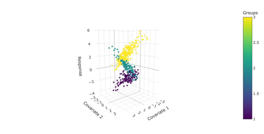
plot2(fit, X, fit$parameters$y_hat, 1, 2)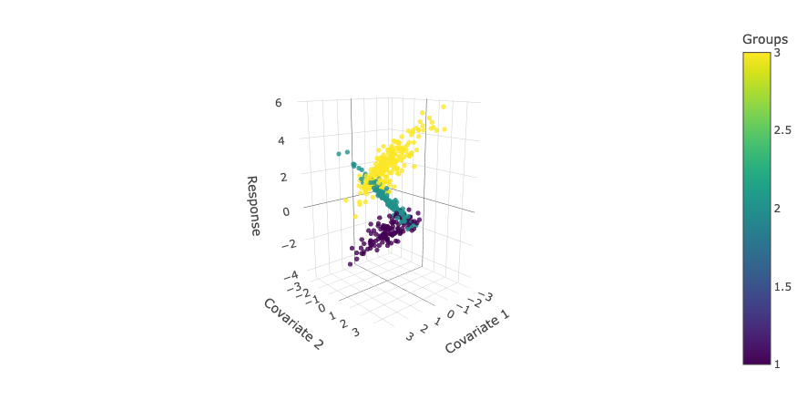
summary() is an S3 method for summarizing results from
the FMRM() and MM_Grid() functions of class
FMRM. Outputs the number of mixture components, optimal lambda-alpha
pair, log-likelihood, ic, mean squared error, and parameters of the
model.
summary(fit)
#> =======================================================================
#> Regularized Finite Gaussian Mixture Regression Model Using MM Algorithm
#> =======================================================================
#>
#> Call:
#>  FMRM(x = X, y = y, G = 4, family = gaussian(), information_criteria = "bic",      parallel = TRUE)
#>
#>  G = 3
#>
#>  lambda = 54.36 || alpha = 1 || log-likelihood = -661.47 ||
#>  BIC  = 1428.6 || MSE = 0.12
#>
#>  Components     1      2      3
#>  Pi           0.237  0.335  0.428
#>  Clusters       123    151    226
#>  Sigma        0.279  0.459  0.384
#>
#>  Beta (Regression Parameters)
#>   Components     1      2      3
#>   Intercept   -1.513  0.502  2.543
#>   Beta 1       0.040  0.984 -1.002
#>   Beta 2       0.990 -0.468  0.492
#>   Beta 3      -0.000  0.179  0.000
#>   Beta 4       0.000  0.000 -0.000
#>   Beta 5       0.029 -0.000 -0.000
#> Beta 6 -0.000 -0.000 -0.031These simulations were carried out in R (version 4.5.0) with RStudio
(version 2026.06.0+242). For benchmarking, the rbenchmark
package was used, found here: https://CRAN.R-project.org/package=rbenchmark. They were
run on a MacBook Air (2022) with an M2 chip, 8 cores (4 performance and
4 efficiency), and 8 GB of memory. The code used to generate the data
used to fit each family of finite mixture regression model is included
below.
set.seed(2025)

# ----Gaussian----

# ----Simulate data----
n <- 500 # total samples
p <- 6 # number of covariates
G <- 3 # number of mixture components
rho = 0.2 # correlation

# ----True parameters for 3 clusters----
betas <- matrix(
  c(
    1,
    2,
    -1,
    0.5,
    0,
    0,
    0, # component 1
    5,
    -2,
    1,
    0,
    0,
    0,
    0, # component 2
    -3,
    0,
    2,
    0,
    0,
    0,
    0 # component 3
  ),
  nrow = G,
  byrow = TRUE
) /
  2
pis <- c(0.4, 0.4, 0.2)
sigmas <- c(0.5, 0.4, 0.3)

# ----Generate correlation matrix----
cor_mat <- outer(1:p, 1:p, function(i, j) rho^abs(i - j))
Sigma <- cor_mat

# ----Simulate design matrix X (n × p)----
X <- mvtnorm::rmvnorm(n, mean = rep(0, p), sigma = Sigma)

# ----Generate responsibilities----
z <- rmultinom(n, size = 1, prob = pis)
groups <- apply(z, 2, which.max)

# ----b0 + b1x1 + b2x2 + ... + bkxp----
mu_vec <- rowSums(cbind(1, X) * betas[groups, ])

# ----Simulate response y----
y <- rnorm(n, mean = mu_vec, sd = sigmas[groups])

# ----Poisson----

# ----Simulate data----
n <- 500 # total samples
p <- 6 # number of covariates
G <- 3 # number of mixture components
rho <- 0.2 # correlation

# ----True parameters for 3 clusters----
betas <- matrix(
  c(
    1,
    2,
    -1,
    0.5,
    0,
    0,
    0, # component 1
    5,
    -2,
    1,
    0,
    0,
    0,
    0, # component 2
    -3,
    0,
    2,
    0,
    0,
    0,
    0 # component 3
  ),
  nrow = G,
  byrow = TRUE
) /
  2
pis <- c(0.4, 0.4, 0.2)

# ----Generate correlation matrix----
cor_mat <- outer(1:p, 1:p, function(i, j) rho^abs(i - j))
Sigma <- cor_mat

# ----Simulate design matrix X (n x p)----
X <- mvtnorm::rmvnorm(n, mean = rep(0, p), sigma = Sigma)

# ----Generate responsibilities----
z <- rmultinom(n, size = 1, prob = pis)
groups <- apply(z, 2, which.max)

# ----b0 + b1x1 + b2x2 + ... + bkxp (log-linear predictor)----
eta_vec <- rowSums(cbind(1, X) * betas[groups, ])

# ----Apply inverse link (exp) to get Poisson means----
mu_vec <- exp(eta_vec)

# ----Simulate response y (count data)----
y <- rpois(n, lambda = mu_vec)

# ----Binomial----

# ----Simulate data----
n   <- 500   # total samples
p   <- 6     # number of covariates
G   <- 3     # number of mixture components
rho <- 0.2   # correlation
m   <- sample(10:30, n, replace = TRUE)  # trials per observation

# ----True parameters for 3 clusters----
betas <- matrix(c(
   0.5,  1.2, -0.8,  0.4,  0.0,  0.0,  0.0,  # component 1
   2.0, -1.0,  0.5,  0.0,  0.3,  0.0,  0.0,  # component 2
  -1.5,  0.0,  1.5,  0.0,  0.0, -0.4,  0.0   # component 3
), nrow = G, byrow = TRUE)
pis <- c(0.4, 0.4, 0.2)

# ----Generate correlation matrix----
cor_mat <- outer(1:p, 1:p, function(i, j) rho^abs(i - j))
Sigma   <- cor_mat

# ----Simulate design matrix X (n x p)----
X <- mvtnorm::rmvnorm(n, mean = rep(0, p), sigma = Sigma)

# ----Generate responsibilities----
z <- rmultinom(n, size = 1, prob = pis)
groups <- apply(z, 2, which.max)

# ----b0 + b1x1 + b2x2 + ... + bkxp----
eta_vec <- rowSums(cbind(1, X) * betas[groups, ])

# ----Apply inverse link (logistic) to get Binomial probabilities----
prob_vec <- plogis(eta_vec)

# ----Simulate response y (successes | failures)----
successes <- rbinom(n, size = m, prob = prob_vec)
y <- cbind(successes, failures = m - successes)| Method | G | Replications | Elapsed (seconds) |
|---|---|---|---|
| Parallel | 3 | 10 | 103.254 |
| Parallel | 4 | 10 | 125.252 |
| Parallel | 5 | 10 | 230.807 |
| Parallel | 6 | 10 | 359.222 |
| Parallel | 7 | 10 | 715.479 |
| Sequential | 3 | 10 | 113.547 |
| Sequential | 4 | 10 | 206.359 |
| Sequential | 5 | 10 | 307.827 |
| Sequential | 6 | 10 | 494.598 |
| Sequential | 7 | 10 | 1107.395 |
| Automatic Stopping | 3 | 10 | 128.178 |
| Automatic Stopping | 4 | 10 | 238.118 |
| Automatic Stopping | 5 | 10 | 262.061 |
| Automatic Stopping | 6 | 10 | 267.270 |
| Automatic Stopping | 7 | 10 | 266.581 |
| Method | G | Replications | Elapsed (seconds) |
|---|---|---|---|
| Parallel | 3 | 10 | 289.525 |
| Parallel | 4 | 10 | 831.046 |
| Parallel | 5 | 10 | 836.103 |
| Parallel | 6 | 10 | 1622.873 |
| Parallel | 7 | 10 | 2265.934 |
| Sequential | 3 | 10 | 326.966 |
| Sequential | 4 | 10 | 1059.252 |
| Sequential | 5 | 10 | 1703.650 |
| Sequential | 6 | 10 | 2757.893 |
| Sequential | 7 | 10 | 3862.902 |
| Automatic Stopping | 3 | 10 | 329.539 |
| Automatic Stopping | 4 | 10 | 1041.354 |
| Automatic Stopping | 5 | 10 | 1219.488 |
| Automatic Stopping | 6 | 10 | 1170.428 |
| Automatic Stopping | 7 | 10 | 1333.859 |
| Method | G | Replications | Elapsed (seconds) |
|---|---|---|---|
| Parallel | 3 | 10 | 107.470 |
| Parallel | 4 | 10 | 380.681 |
| Parallel | 5 | 10 | 873.549 |
| Parallel | 6 | 10 | 1646.376 |
| Parallel | 7 | 10 | 2815.387 |
| Sequential | 3 | 10 | 121.764 |
| Sequential | 4 | 10 | 423.203 |
| Sequential | 5 | 10 | 1113.758 |
| Sequential | 6 | 10 | 2327.621 |
| Sequential | 7 | 10 | 3801.199 |
| Automatic Stopping | 3 | 10 | 117.798 |
| Automatic Stopping | 4 | 10 | 447.627 |
| Automatic Stopping | 5 | 10 | 445.004 |
| Automatic Stopping | 6 | 10 | 419.762 |
| Automatic Stopping | 7 | 10 | 437.278 |